Chapter 4

Chapter 4: A Finite Deformable Boundary Cosmology

Chapter 4 figure anchors

Figure 4-1 Figure 4-2 Figure 4-3 Figure 4-4 Figure 4-5 Figure 4-6

Abstract

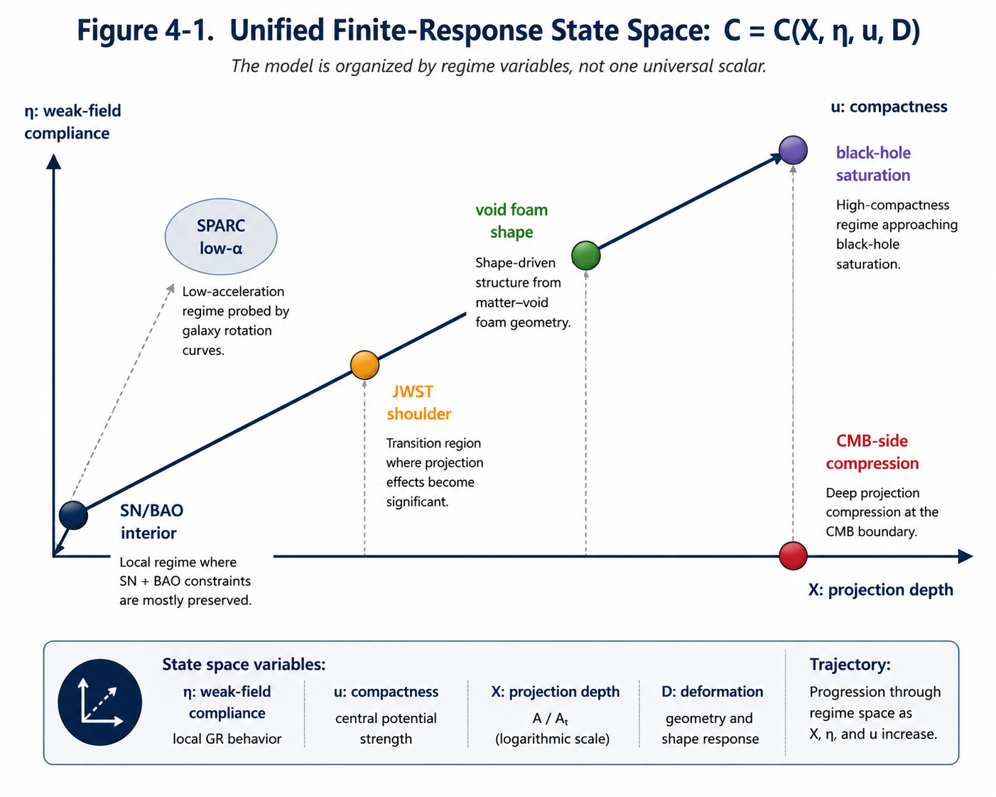
This chapter defines a finite deformable boundary cosmology. In this model, local gravity is preserved as a General-Relativity-compatible limit, while cosmological observations are interpreted through separate internal registers rather than a single universal expansion scale. The universe is treated as a bounded deformable event-domain characterized by an interior stable region, an approach regime, a projection boundary, and a compressed projection side, alongside local deformation wells and matter-void foam.

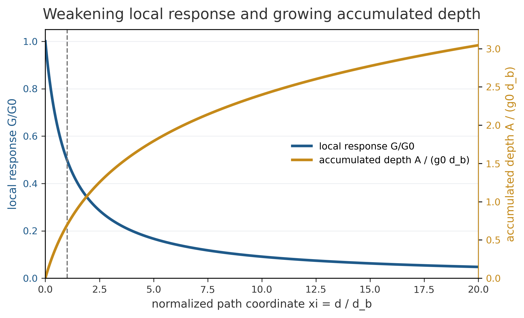
Observed redshift is maintained as the direct observable but is expressed as accumulated path response, \(A = \ln(1 + z)\). The response law \(G(d) = g_0/(1 + d/d_b)\) integrates to \(A(d) = g_0 d_b \ln(1 + d/d_b)\), establishing a non-expansion path coordinate \(d(z)\). Observable distances are subsequently split into radial, transverse, luminosity, angular-size, time-stretch, acoustic, morphology, gravity, and compactness registers.

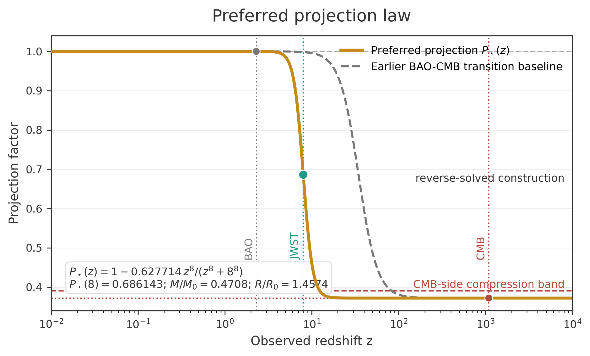
The preferred projection law, \(P_{\star}(z) = 1 - 0.627714 z^8/(z^8 + 8^8)\), is derived from three primary observational anchors: the preservation of the BAO range, the mass-size shifts observed in JWST galaxies, and the compressed projection band of the CMB. This resulting construction leaves the BAO range nearly unchanged, shifts the inferred properties of \(z \approx 8\) galaxies, and approaches the same CMB-side compression identified by the BAO-CMB shared-ruler failure. The completed model is a finite-register cosmology: local GR behavior remains intact, path-response redshift governs the interior, a projection shoulder exists in the high-redshift regime, and a compressed acoustic projection register defines the CMB boundary.

The register-scaling constants \(K_D \sim 1/2\), \(K_X \sim 1\), and \(K_\eta \sim 2/3\) provide a compact test of whether the finite-register sectors behave as unrelated adjustments or as linked scaling regimes of one deformable geometry. The compactness test remains inconclusive, so the full cosmology adopts \(K_u=1/3\) as the working compactness exponent, with \(K_u\sim0\) retained as the saturation-threshold alternative.

Reader note: The final model keeps local gravity in its familiar form and treats deep-cosmos observations as different ways of reading one finite setting. Redshift builds along the light path, galaxy sizes and masses depend on how observations are translated, and the oldest-light scale marks the compressed side of the proposed boundary behavior.

1. Cosmological Premise

The model begins with the premise that measurement is internal to the universe [73]. Before a universe-state exists, concepts such as size, duration, distance, and direction have no operational meaning. Once a finite event-domain is established, clocks, rulers, wavelengths, and structures become meaningful from within that domain. Consequently, the universe is described as a finite deformable geometry whose observables are read from the inside, rather than as an object expanding against an external ruler.

This chapter integrates the components developed previously. The redshift sector utilizes the path-response law \(A(d)=\ln(1+z)\), while the observational sector provides the finite-depth coordinates and projection registers. The synthesis organizes projection, gravity, morphology, and compactness through the variables \(X, \eta, u,\) and \(D_n\).

Key symbols used throughout the model are summarized on the Measurement Registers page.

**Figure 4-1.** Finite deformable boundary cosmology. The universe is represented as a bounded event-domain with an interior stable register, an approach/JWST shoulder, a projection boundary, a compressed CMB-side projection register, local deformation wells, matter-void foam, and compactness screens.

2. Local Gravity as the Interior Boundary Condition

To ensure the model remains physically viable, it must first be proven that it does not break the laws of physics we have already verified in our own solar system. Therefore, the interior stable register is designed to match General Relativity in the local, weak-field limit. In this regime, a spherical mass is represented by a three-dimensional spatial deformation and a coupled local clock-rate field. The spatial line element is expressed as:

\[d\ell^2 = \psi^4(r)\left(dr^2 + r^2d\Omega^2\right),\quad \psi(r) = 1 + \frac{GM}{2c^2r} \tag{4-1}\]

The clock-rate field follows the same deformation:

\[dT = \alpha(\psi)d\tau,\quad \alpha(\psi) = \frac{2 - \psi}{\psi} \tag{4-2}\]

Substitution yields:

\[\alpha(r) = \frac{1 - GM/(2c^2r)}{1 + GM/(2c^2r)} \tag{4-3}\]

Equations (4-1) through (4-3) reproduce the isotropic Schwarzschild exterior form when written as three-dimensional space with a lapse-like local time factor. In the weak-field expansion, the effective post-Newtonian parameters are \(\beta = 1\) and \(\gamma = 1\). This ensures the model maintains the standard local solar-system limit used for light deflection, Shapiro delay, redshift, and perihelion advance [74] [75].

See the Quantitative Appendix for the local weak-field expansion note.

This defines the role of space and time in the model. Space is the deformable three-dimensional domain, while time is a positive local ordering of physical change. While they are distinct dimensions, local observations require the clock-rate register to remain coupled to the spatial deformation.

3. Model Definition

Definition 4.1. A finite deformable boundary cosmology consists of the following linked structures:

3.1 Local 3D-plus-Clock Gravity

\[d\ell^2 = \psi^4(r)\left(dr^2 + r^2d\Omega^2\right),\quad \psi(r)=1+\frac{GM}{2c^2r},\quad dT=\frac{2-\psi}{\psi}d\tau \tag{4-4}\]

This defines the interior gravitational limit and is not re-fit cosmologically.

3.2 Cosmological Path Response

Rather than viewing redshift as a result of space expanding, this model treats it as a record of the total interaction a photon has with the geometry of the path it traveled. The response is defined by the integral of a local rate over the path distance:

\[A(d) = \int_0^d G(s)\,ds,\quad G(d)=\frac{g_0}{1+d/d_b} \tag{4-5}\]

In this expression, \(d\) and \(d_b\) share distance units, \(g_0\) has inverse-distance units, and \(p = g_0d_b\) is dimensionless.

See the Quantitative Appendix for finite-response inversion and units.

\[A(d)=g_0 d_b \ln(1+d/d_b) \tag{4-6}\]

Technical note

Since \(A = \ln(1+z)\), the inverse finite path coordinate is:

\[d(z)=d_b\left[(1+z)^{1/(g_0 d_b)}-1\right] \tag{4-8}\]

Technical note

With \(p = g_0 d_b\) and \(\xi = d/d_b\):

\[\xi(z)=\exp\left[A(z)/p\right]-1 = (1+z)^{1/p}-1 \tag{4-10}\]

**Figure 4-2.** Path response. The local contribution \(G\) weakens as the normalized path coordinate \(\xi\) increases, while the accumulated response \(A\) continues to grow.

3.3 Register-Split Cosmological Distances

Rather than forcing all observables into one universal register, the model separates distances into specific roles:

\[D_R(z)=d(z),\quad D_H(z)=\frac{dD_R}{dz},\quad D_M(z)=d(z) \tag{4-11}\]

The finite-model radial register is written as \(D_H = dD_R/dz\), which is equivalent to \(c/H_{\text{eff}}(z)\) if an effective Hubble register is defined. This is distinct from the standard \(\Lambda\text{CDM} H(z)\).

\[D_L(z)=(1+z)^{q_L}D_M(z),\quad D_A(z)=\frac{D_M(z)}{(1+z)^{q_A}} \tag{4-12}\]

The empirical luminosity register yields \(q_L \approx 1.233\text{ to }1.2335\) when \(p \approx 19.878\) is anchored by the BAO radial/transverse shape. While standard metric distance-duality corresponds to \(q_L=1\) when \(q_A=1\) [76] [77], the finite model interprets \(q_L \neq 1\) as a real luminosity/time-transfer projection effect.

3.4 Reverse-Solved Projection Law

The projection law is derived by working backward from the observed boundaries of the universe. Think of this as a "reverse-engineering" process: the law is constructed specifically to satisfy three primary observational anchors: the preservation of the BAO range, the JWST mass-size estimates, and the CMB compression band.

\[P_{\star}(z)=1-\frac{\Delta z^n}{z^n+z_s^n},\quad \Delta=0.627714,\quad z_s=8,\quad n=8 \tag{4-13}\]

\[P_{\star}(z)=1-\frac{0.627714 z^8}{z^8+8^8} \tag{4-14}\]

This construction is used as the organized projection target. This approach aligns with conformal methods in cosmology, where metric rescalings preserve angular structure while altering length-scale relations [1] [82]. While distinct from a direct conformal transformation of the metric, the model uses empirical finite-register mappings to organize distance, angular-size, and acoustic-scale behavior.

See the Quantitative Appendix for projection-transition definitions and stage diagnostics.

**Figure 4-4.** Preferred projection law. \(P_{\star}(z)\) preserves the BAO regime, modifies the JWST \(z \approx 8\) register, and approaches the CMB-side compressed projection band.

3.5 Finite-Deformation Curvature Bridge

To connect these registers to the underlying geometry, the local three-dimensional curvature relation is extended by a finite-response correction:

\[{}^3R[h] = \frac{16\pi G}{c^2}\rho F(X) + L_F^{-2} Q(X) \tag{4-15}\]

\(F(X)\) and \(Q(X)\) are dimensionless response functions, and \(L_F\) is a finite-response length scale. In the local limit:

See the Quantitative Appendix for curvature-bridge definitions and response-register notation.

\[F(X) \rightarrow 1, \quad Q(X) \rightarrow 0 \quad \text{for } X \ll 1. \tag{4-17}\]

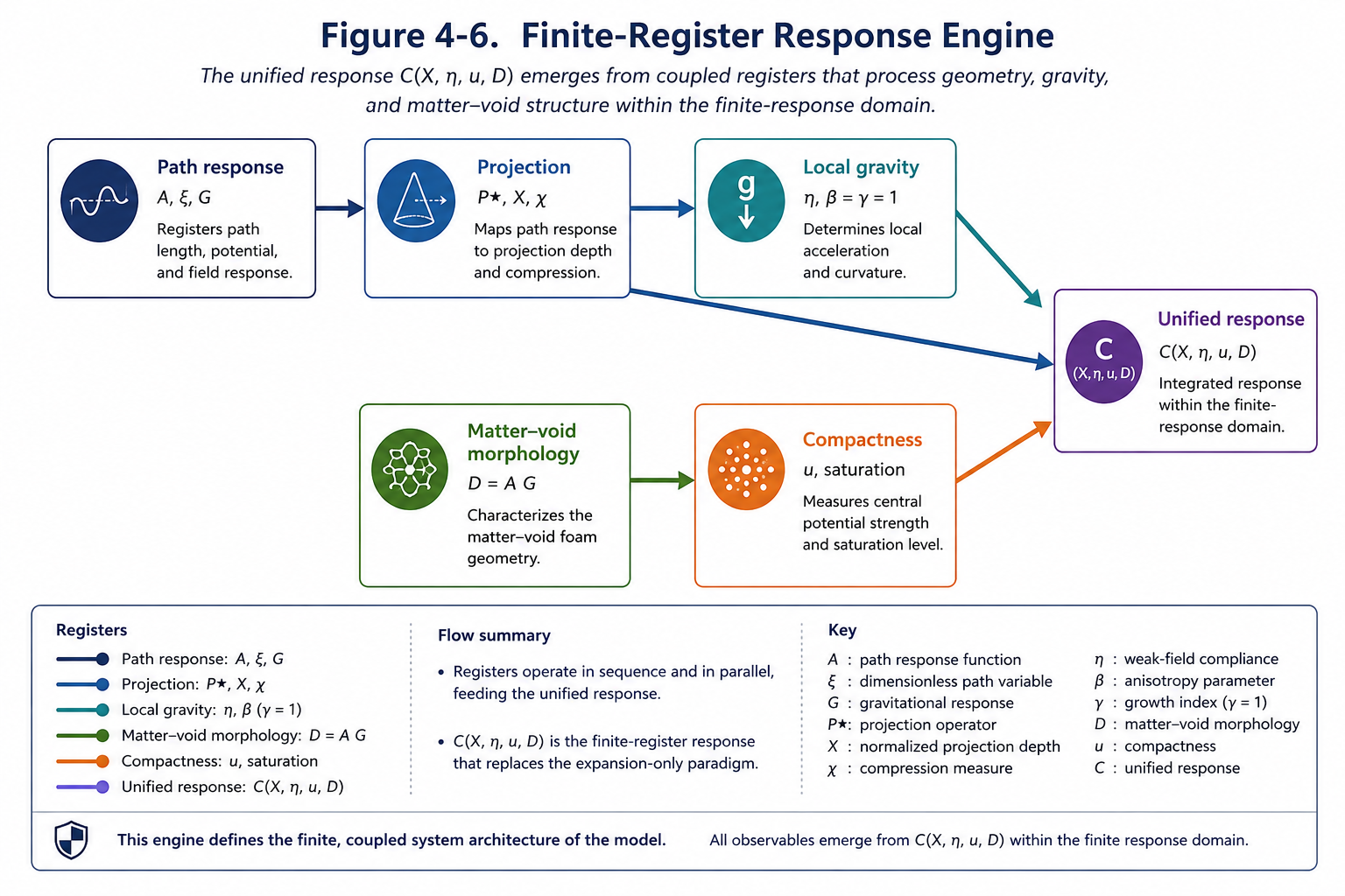
The long-term theoretical target is a unified response engine:

\[C = C(X,\eta,u,D_n) \tag{4-16}\]

Technical note

Here, \(X\) is projection depth, \(\eta\) is weak-field gravity compliance, \(u\) is compactness, and \(D_n = D/D_0\) is the normalized matter-void morphology coordinate.

4. Dimensionless Finite-Register Dictionary

The model employs dimensionless registers to keep measurement scales distinct. Redshift is measured directly and then mapped into several specialized coordinates, as shown in Figure 4-3.

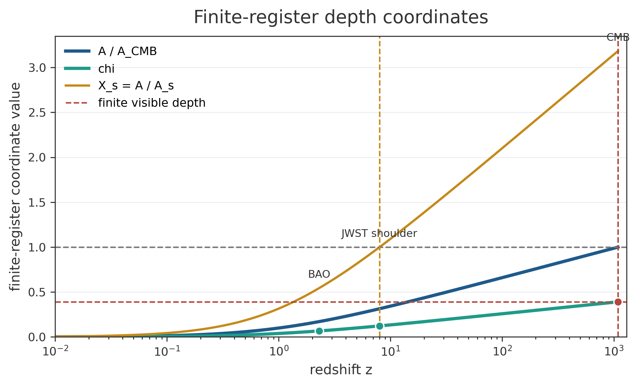
**Figure 4-3.** Redshift recast into finite-register depth coordinates. \(A/A_{\mathrm{CMB}}\), \(\chi\), and \(X\) are related but not interchangeable.

Table 4-1. Dimensionless finite-register dictionary.

Register	Definition	Role
\(z\)	Observed redshift	Measured spectral shift
\(A = \ln(1+z)\)	Accumulated path response	Redshift bookkeeping register
\(\xi = d/d_b\)	Normalized path coordinate	Finite path depth from the response solution
\(G = 1/(1+\xi)\)	Local response rate	Weakening incremental response
\(X = A/A_s\)	Projection-depth coordinate	\(X=1\) at the preferred JWST-centered projection shoulder
\(\chi = f_{\mathrm{vis}} A/A_{\mathrm{CMB}}\)	Finite-depth display coordinate	Places BAO, JWST, and CMB on one compact depth scale
\(D = AG\)	Morphology response	Raw matter-void foam coordinate
\(D_n = D/D_0\)	Normalized morphology response	Response-function argument; \(D_0\) shares units with \(D\)
\(\eta = g_{\mathrm{bar}}/g^\dagger\)	Weak-field gravity coordinate	SPARC/RAR-style compliance register
\(u = 2GM/(Rc^2)\)	Compactness coordinate	Black-hole/finite-saturation register
\(P_{\star}(z)\)	Projection factor	Mass-size/acoustic projection conversion

5. Register Scaling Constants and Response Weighting

The finite-register dictionary separates the observables. The scaling constants show how those registers enter the response engine as distinct weights:

\[D_n^{K_D}, \qquad X^{K_X}, \qquad \eta^{K_\eta}, \qquad u^{K_u}\]

With \(K_D \sim 1/2\), the matter-void register behaves like a square-root transport response. With \(K_X \sim 1\), the projection coordinate remains nearly proportional through the interior and approach regime. With \(K_\eta \sim 2/3\), the weak-field gravity register behaves like a dimensional-coupling response. The compactness-sector test was attempted but did not yet recover a clear \(K_u\); for the full cosmology, \(K_u=1/3\) is used as the working radial-collapse exponent. The alternate outcome is \(K_u\sim0\), where compactness behaves as a saturation switch rather than a broad scaling register.

\[C_{\mathrm{scaled}} = C\left(X^{K_X},\eta^{K_\eta},u^{K_u},D_n^{K_D}\right),\quad K_u=\frac{1}{3}\]

This is the diagnostic scaling form of the response engine. It does not replace the curvature bridge or the projection law; it records how the register constants enter the finite-boundary cosmology as measurable structure and as explicit future tests.

Table 4-2. Register scaling weights.

Register	Scaled form	Recovered behavior	Cosmological role
Matter-void morphology	\(D_n^{K_D}\)	\(K_D \sim 1/2\)	Transport-like foam response
Projection depth	\(X^{K_X}\)	\(K_X \sim 1\)	Coherent interior-to-shoulder ordering
Weak-field compliance	\(\eta^{K_\eta}\)	\(K_\eta \sim 2/3\)	Dimensional coupling in galaxy-scale response
Compactness	\(u^{K_u}\)	working \(K_u=1/3\); alternate \(K_u\sim0\)	Radial collapse scaling with saturation-threshold test

6. Reverse-Solved Projection as the Organizing Construction

The projection law is fixed by working backward from specific observational anchors. The BAO requires the low-redshift acoustic-shape range to remain nearly unchanged. The JWST requires the high-redshift galaxy conversion to shift stellar mass downward and effective radius upward. Finally, the CMB requires the far-side acoustic projection to approach the compressed scale identified by the BAO-CMB shared-ruler failure. This is why \(P_{\star}\) is treated as the organizing construction for the cosmology, while its physical derivation remains a primary model-building target.

Earlier transitions placed the midpoint near \(z_t \approx 34.6\). While that transition reached the CMB-side compression, it was nearly unity at \(z \approx 8\) and thus did not alter JWST galaxy sizes. The reverse solution shifts the projection shoulder into the JWST regime while increasing sharpness to preserve the BAO range.

Table 4-3. Anchor values for the preferred projection law \(P_{\star}\).

Regime	\(z\)	\(A = \ln(1+z)\)	\(\chi\)	\(P_{\star}\)	Mass ratio \(P^2\)	Radius ratio \(1/P\)
BAO high end	2.3	1.1939	0.0667	0.999971	0.9999	1.0000
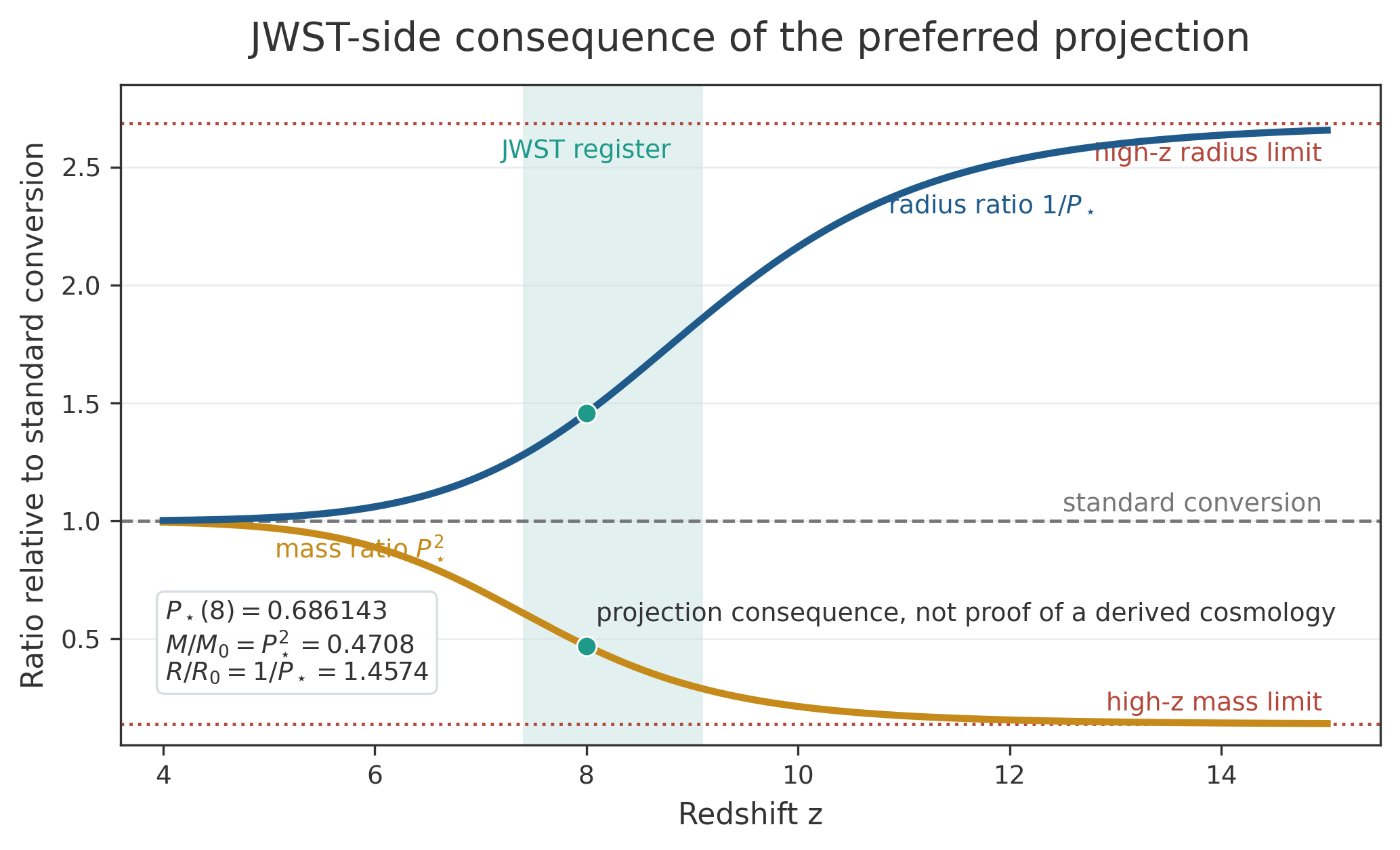
JWST shoulder	8	2.1972	0.1228	0.686143	0.4708	1.4574
CMB side	1089.92	6.9948	0.3909	0.372286	0.1386	2.6861

At \(z = 2.3\), \(P_{\star} = 0.999988\), meaning the BAO range is nearly unchanged. At \(z = 8\), \(P_{\star} = 0.686143\). In the JWST mass-size register, this implies \(M_{\text{new}}/M_{\text{standard}} \approx P_{\star}^2 \approx 0.4708\) and \(R_{\text{new}}/R_{\text{standard}} \approx 1/P_{\star} \approx 1.457\). At \(z = 1089.92\), \(P_{\star}\) approaches 0.372286, matching the compressed asymptote required by the CMB-side projection band.

**Figure 4-5.** JWST consequence of \(P_{\star}\). The preferred projection law lowers inferred stellar mass and increases inferred effective radius in the \(z \approx 7\)–\(9\) high-redshift galaxy regime.

7. Observable Sectors of the Cosmology

7.1 Redshift and Supernova Luminosity

The supernova sector utilizes the path-response solution and luminosity register. Redshift is treated as \(A = \ln(1+z)\), the radial path coordinate is \(d(z)\), and observed brightness is compared through \(D_L = (1+z)^{q_L} D_M\). This effectively separates spectral shift, finite path length, and luminosity transfer. Consequently, the supernova curvature that motivated Chapter 1 is preserved as the interior path-response sector of the cosmology.

7.2 BAO Radial/Transverse Shape

The BAO anisotropy sector uses the register ratio:

\[Q_{\mathrm{BAO}}(z)=\frac{D_M(z)}{D_H(z)} \tag{4-18}\]

Since the absolute ruler scale \(r_d\) cancels from \(\Delta z/\theta\) (as shown in Chapter 1), this sector compares the shape of radial and transverse distances before imposing a shared acoustic calibration. The finite model uses the same path coordinate \(d(z)\) for \(D_M\) and the derivative register \(dD_R/dz\) for \(D_H\).

7.3 BAO-CMB Acoustic Projection

The BAO-CMB shared-ruler failure is represented as a projection-boundary effect rather than a failure of local gravity. \(P_{\star}\) leaves the BAO redshift range nearly unchanged while shifting the CMB-side register toward the high-redshift compressed band. The near-unity scaling \(K_X \sim 1\) is consistent with this behavior: the interior projection order is preserved while the boundary-side acoustic register compresses.

7.4 Time Dilation

Technical note

The time-stretch sector follows from the same accumulated response. Since \(A = \ln(1+z)\), arrival intervals stretch as:

\[\Delta t_{\mathrm{obs}} = \Delta t_{\mathrm{em}} e^A = \Delta t_{\mathrm{em}}(1+z) \tag{4-20}\]

Technical note

The model therefore predicts the standard \(b=1\) time-dilation exponent, interpreting the stretching as a path-response timing register rather than as evidence that all registers must share a single FLRW expansion scale.

7.5 High-Redshift Galaxy Mass and Size

JWST high-redshift galaxies serve as direct tests of derived quantities. While spectroscopic redshift, flux, and angular size are direct observables, stellar mass, luminosity, physical size, and compactness are inferred through cosmological conversion. In the finite projection register, the leading conversion is:

\[M_{\star,\text{FD}} \approx P_{\star}^2 M_{\star,\text{standard}}, \quad R_{e,\text{FD}} \approx R_{e,\text{standard}}/P_{\star} \tag{4-21}\]

Flux-based inferred mass scales with luminosity-distance squared, while physical radius scales through the angular-size-distance register. The projection factor is used here as a diagnostic scaling (see the quantitative appendix). Thus, the same projection shoulder that preserves BAO and reaches the CMB-side limit moves \(z \approx 8\) galaxy properties toward lower inferred mass, larger radius, and lower compactness.

See the Quantitative Appendix for the diagnostic mass-size scaling details.

7.6 Weak-Field Gravity

The galaxy-scale gravity register uses:

\[\eta = \frac{g_{\mathrm{bar}}}{g^\dagger} \tag{4-22}\]

The corresponding compliance function is written as:

\[C_g(\eta)=1-\exp\left(-\sqrt{\eta}\right) \tag{4-23}\]

This register integrates low-acceleration galaxy behavior into the finite-response vocabulary without altering the local high-acceleration GR-compatible limit. The associated \(K_\eta \sim 2/3\) scaling identifies the weak-field sector as a dimensional-coupling response.

7.7 Matter-Void Morphology

The matter-void sector employs:

\[D = A\,G,\quad D_n = D/D_0 \tag{4-24}\]

This register treats the cosmic web as a matter-plus-void foam, rather than merely a distribution of matter points. \(D\) combines the accumulated path response with the local weakening rate to provide the raw morphology coordinate developed in previous chapters. With \(K_D \sim 1/2\), the morphology sector enters the response engine as a transport-like weakening-response register.

7.8 Compactness and Finite Saturation

The compactness sector uses:

\[u = \frac{2GM}{Rc^2} \tag{4-25}\]

In the finite-domain interpretation, \(u\) is a regime coordinate that approaches saturation rather than literal physical infinity. Singular behavior marks the edge of a response law's domain, not the required existence of infinite physical density.

The compactness-sector test attempted with available black-hole mass and lag-radius data was not decisive. For the model definition, the compactness register is therefore assigned the working exponent \(K_u=1/3\), representing radialized collapse scaling. If future data instead favor \(K_u\sim0\), compactness would be interpreted as a saturation-threshold register rather than a scaling register.

8. Unified Finite-Response Engine

The finite-boundary cosmology is not a collection of unrelated corrections; its observable sectors are faces of a single deformable domain. Projection depth, path response, weak-field gravity, foam morphology, compactness, and register scaling are integrated into the response engine:

\[C = C(X, \eta, u, D_n),\quad C_{\mathrm{scaled}} = C\left(X^{K_X},\eta^{K_\eta},u^{K_u},D_n^{K_D}\right),\quad K_u=\frac{1}{3} \tag{4-26}\]

The curvature bridge, projection law, and observational registers are connected via:

\[{}^3R[h] = \frac{16\pi G}{c^2}\rho F(X) + L_F^{-2}Q(X) \tag{4-27}\]

\(F\) and \(Q\) are components or limiting cases of the broader finite-response function \(C(X, \eta, u, D_n)\). In the local regime, \(F \rightarrow 1\) and \(Q \rightarrow 0\). The finite-boundary regime activates projection, morphology, weak-field, and compactness scaling registers without altering local laboratory or solar-system physics.

**Figure 4-6.** Unified finite-response engine. The observable registers are treated as linked responses of one finite deformable domain, with \(K_D\), \(K_X\), \(K_\eta\), and working \(K_u=1/3\) supplying the register-scaling weights.

9. Cosmological Picture

The resulting universe is a finite deformable boundary system. Its interior is locally stable and GR-compatible. Redshift accumulates as path response rather than as a direct reading of a universal expansion scale. BAO radial/transverse shape follows the interior path register. At greater finite depth, the projection shoulder appears in the high-redshift galaxy regime, altering inferred mass and size. Beyond that, the acoustic projection approaches the CMB-side compressed register.

This framework explains why different observables can agree locally yet diverge globally. A clock, a wavelength, a ruler, an angular size, a luminosity, a void shape, a galaxy rotation curve, and a compactness boundary are all internal measurements, but they do not necessarily remain locked to a single background scale across the full finite domain.

The model's central physical claim is that the universe does not require an infinite external stage or a single universal measurement register. Instead, it is a finite deformable event-domain where internal observables separate into stable local registers, approach registers, projection registers, and compressed boundary registers.

10. Empirical Correspondence

Table 4-4. Empirical correspondence of the finite-boundary cosmology.

Sector	Register	Scaling behavior	Model Role
Local gravity	3D+clock exterior	ordinary high-acceleration limit	\(\beta=1, \gamma=1\) weak-field limit
Supernovae	\(A(d), d(z), D_L\)	path-response sector; no independent \(K\) isolated	nonlinear redshift-distance curvature as path response
BAO shape	\(D_M/D_H\)	linked to \(K_X \sim 1\)	radial/transverse anisotropy without absolute-ruler dependence
BAO-CMB	\(P_{\star}\) high-z asymptote	projection compression after coherent interior ordering	compressed acoustic projection band
JWST galaxies	\(P_{\star}\) mass-size conversion	projection-shoulder response	lower mass, larger radius, lower compactness
Time dilation	A timing register	inherits \(A=\ln(1+z)\)	\(\Delta t_{\text{obs}}=\Delta t_{\text{em}}(1+z)\)
SPARC/RAR	\(\eta\)	\(K_\eta \sim 2/3\)	weak-field compliance register
Voids/foam	\(D=AG\)	\(K_D \sim 1/2\)	matter-void morphology register
Compactness	\(u\)	working \(K_u=1/3\); alternate \(K_u\sim0\)	finite saturation register with radial collapse scaling

From a model-building perspective, the structural form is now fixed: local GR-compatible gravity, accumulated path response, register-split distances, the reverse-solved projection construction \(P_{\star}\), the register-scaling constants \(K_D\), \(K_X\), \(K_\eta\), the working compactness exponent \(K_u=1/3\), and the unified response engine \(C(X, \eta, u, D_n)\). Further development focuses on precision implementation and physical derivation rather than the invention of the cosmological structure.

11. Definition and Status of the Finite-Boundary Model

The finite deformable boundary cosmology is defined by six fundamental statements:

1. The universe is a finite deformable event-domain, rather than an object measured from an external infinite ruler.

2. Local gravity is the GR-compatible interior limit, expressed as three-dimensional spatial deformation plus a coupled positive clock-rate field.

3. Observed redshift is accumulated path response:

\[A=\ln(1+z),\quad G(d)=\frac{g_0}{1+d/d_b}. \tag{4-28}\]

4. Cosmological observables occupy separate but linked finite registers: \(D_R, D_H, D_M, D_L, D_A\), timing, acoustic projection, morphology, gravity compliance, and compactness.

5. The preferred projection construction is fixed by BAO preservation, JWST mass-size conversion, and CMB-side compression:

\[P_{\star}(z)=1-\frac{0.627714 z^8}{z^8+8^8}. \tag{4-29}\]

6. The full finite-response engine uses register scaling, with recovered values \(K_D\sim1/2\), \(K_X\sim1\), and \(K_\eta\sim2/3\), and with compactness assigned the working value \(K_u=1/3\):

\[C_{\mathrm{scaled}} = C\left(X^{K_X},\eta^{K_\eta},u^{1/3},D_n^{K_D}\right). \tag{4-30}\]

The register-scaling result changes the status of the model. The finite-register framework is not only a way to keep observables separated; it now contains a quantitative signature. The recovered constants \(K_D \sim 1/2\), \(K_X \sim 1\), and \(K_\eta \sim 2/3\) place morphology response, projection depth, and weak-field compliance into different scaling regimes of one deformable system. The compactness-sector test was attempted but remains inconclusive, so \(K_u=1/3\) is used as a working definition for radial collapse scaling. A future model must explain not only the individual observational fits, but why these registers favor a low-order exponent family.

The model matches local weak-field gravity by construction, reproduces the path-response redshift sector, preserves the BAO radial/transverse regime, shifts JWST high-redshift mass-size inferences in the required direction, and reaches the CMB-side compressed projection band. Remaining quantitative development includes full covariance likelihoods, a complete CMB-spectrum implementation, homogeneous JWST population remeasurement, numerical evolution of the unified response engine, and a stronger compactness-sector test of \(K_u=1/3\) against the \(K_u\sim0\) saturation-only alternative.

The cosmology is therefore a defined finite-register model of a universe with stable local behavior, finite-depth path response, a projection shoulder, and a compressed boundary-side register.

Reader note: The closing model is defined enough to be tested, but not complete. Its next burden is to show the same behavior with stronger statistics, full oldest-light modeling, consistent JWST measurements, and a physical explanation for the proposed transition.