Chapter 2
Chapter 2: Observational Registers: Galaxies, Gravity, Voids, and Boundaries
Chapter 2 figure anchors
Abstract
The finite deformable redshift framework is extended here across additional observational registers. A previously identified BAO-CMB shared-ruler failure established a sharp recovery transition. Recasting this result as a dimensionless projection-depth scale yields \(\chi\), defined from the CMB-to-BAO separate-scale ratio of 0.390906. This coordinate places the BAO regime in the transparent interior, JWST \(z \approx 8\) galaxies on the approach to the transition, the reconstructed projection break near \(\chi \approx 0.20\), and the CMB-side scale near \(\chi \approx 0.39\). These values represent normalized depth coordinates and are distinct from the accumulated response \(A = \ln(1+z)\) or redshift itself.
An evaluation of Labbé-Baggen JWST data demonstrates that a finite-geometry projection shoulder shifts published \(z > 7\) galaxy properties toward lower inferred stellar mass, larger effective radius, and lower compactness. An expanded JWST-PRIMAL spectroscopic analysis does not isolate a clean residual color or sky-position signal after accounting for line strength, ionization, Ly\(\alpha\) damping behavior, and UV slope. The gravitational extension incorporates the SPARC radial acceleration relation, selected dissociative cluster offsets, and large-scale basins of attraction. The most definitive gravitational result is the galaxy-scale acceleration transition: SPARC binned data recover a characteristic acceleration near \(10^{-10}\) m s\(^{-2}\), where the observed-to-baryonic response rises systematically below that scale.
An SDSS DR7 VAST morphology screen evaluates whether matter-void foam architecture is better organized by the full finite-response coordinate \(D = AG\) than by redshift or \(A = \ln(1+z)\) alone. While \(D\) improves several independent shape metrics, standard redshift remains competitive, and the SDSS depth is insufficient to reach the proposed transition range. The field-equation bridge retains general relativity as the local high-acceleration limit while adding a finite-geometry correction term that activates near regime thresholds. Finally, the black-hole extension treats \(u = 2GM/(Rc^2)\) as a compactness-regime variable that approaches finite saturation rather than physical infinity.
Keywords: JWST, high-redshift galaxies, finite geometry, redshift, BAO-CMB tension, projection effects, PRIMAL, DAWN JWST Archive, SPARC, radial acceleration relation, galaxy clusters, basins of attraction
The organizing premise is that the universe may not possess a common measurement scale across all registers. Redshift, luminosity distance, angular-size distance, weak-field gravity, void architecture, and compactness may remain locally measurable while requiring distinct finite-response coordinates when compared across different regimes.
1. Introduction
A redshift path-response analysis previously examined whether redshift could be treated as an accumulated response inside a finite deformable geometry, rather than as a purely expansion-based distance clock. This analysis established that while the supernova redshift-distance relation can be represented by a compact declining-response law, the mapping fails when BAO and CMB information are forced to share a single acoustic-ruler calibration. The resulting recovery target preserved the low- and intermediate-redshift BAO range while rapidly changing the high-redshift projection.
High-redshift JWST galaxies provide an independent domain to test this conversion issue. The critical distinction lies between direct observables and cosmology-dependent derived quantities. Spectroscopic redshift, observed flux, sky position, line ratios, and continuum slopes are direct measurements. Conversely, stellar mass, physical radius, luminosity, star-formation rate, age, and number density require a cosmological conversion from redshift to distance and time. If this conversion is incomplete at high redshift, galaxies may appear erroneously massive, compact, or old, even when the measured spectra are correct.
This analysis evaluates whether derived masses, sizes, colors, and sky/redshift structures behave in a manner compatible with a projection-register shift. Mass-size quantities shift in the direction predicted by a finite-geometry projection correction; however, spectral color and sky-position structure do not show a clear residual geometric signal in the present PRIMAL tests.
2. Dimensionless Finite-Geometry Depth Coordinate
The BAO-CMB analysis identified an effective separate-scale ratio between CMB-side and BAO-side acoustic calibration. Let \(S_{\mathrm{BAO}}\) be the effective BAO-side calibration scale and \(S_{\mathrm{CMB}}\) the effective CMB-side calibration scale. Their ratio serves as the organizing depth scale. The visible-to-total finite-geometry radius fraction is defined as:
See the Quantitative Appendix for the separate-scale ratio and calibration details.
This ratio yields a total-to-visible radius ratio of 2.558 and a visible-to-total volume fraction of 0.0597. It also produces an attenuation-like value, \(-\ln(f_{\mathrm{vis}}) = 0.939\), which is close to one optical-depth unit. This ratio is employed here as a dimensionless depth coordinate:
Equation (2-2) maintains redshift as the measured quantity while mapping it onto a compact depth scale. With \(z(\text{CMB}) = 1089.92\), the CMB-side scale lies at \(\chi = 0.390906\) by construction. Lower redshift observables consequently occupy smaller positions within this finite-geometry depth.
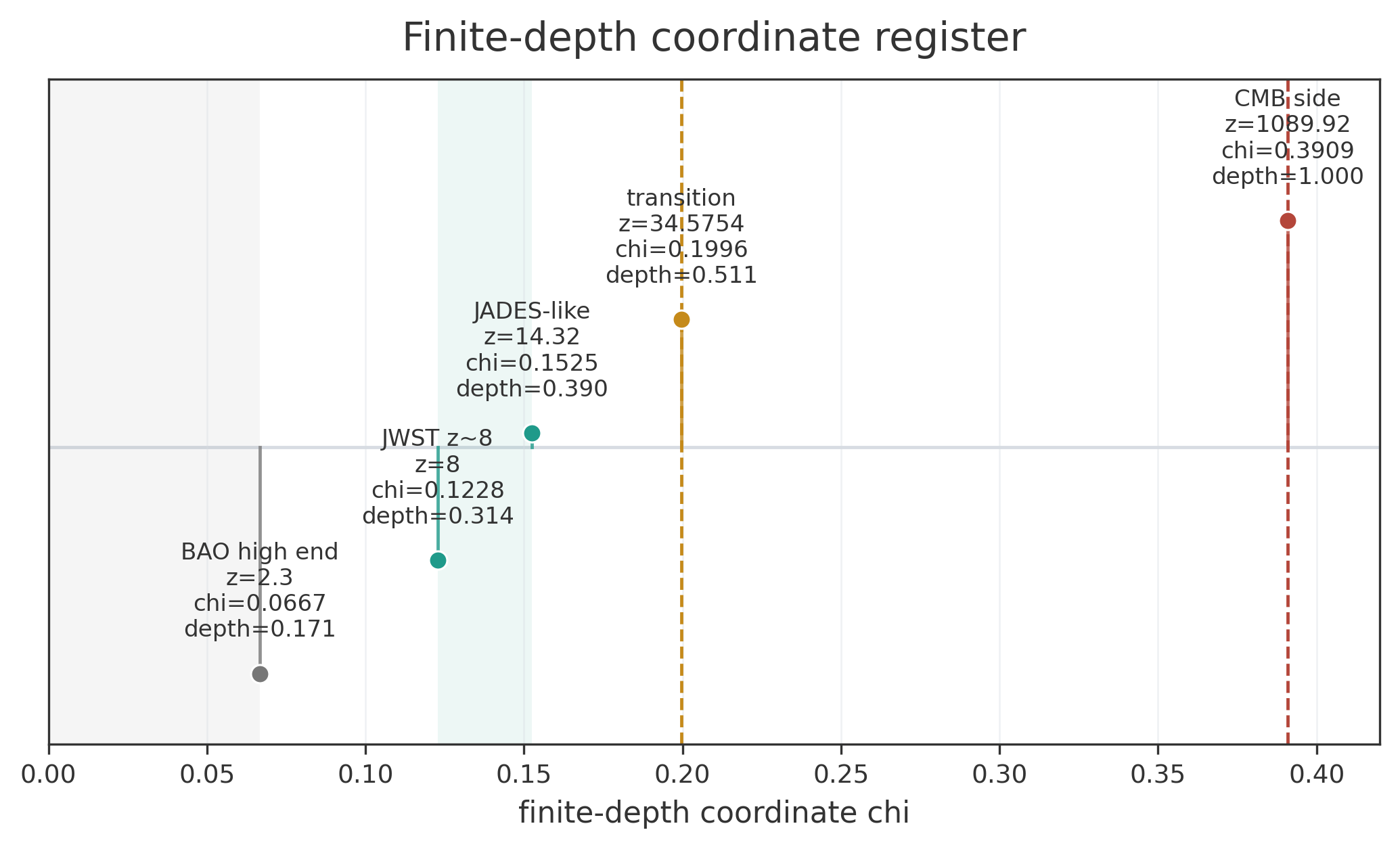
Coordinate discipline is essential. The redshift-response analysis utilized \(A = \ln(1+z)\) as the accumulated path response and \(G(d)\) as the local response rate. The \(\chi\) coordinate is a finite-depth display coordinate scaled by the CMB-to-BAO separate-scale ratio. While related, these quantities are not interchangeable. The normalized transition coordinate \(X = A/A_t\), where \(A_t = \ln(1+z_t)\) and \(z_t = 34.5754\), provides a common comparison coordinate. In this notation, \(X = 1\) marks the reconstructed recovery transition, analogous to a one-focal-length transition scale.
Table 2-1. Key observables recast onto the dimensionless finite-geometry depth scale.
| Symbol or Value | Definition | Use in Finite-Response Analysis |
|---|---|---|
| \(z\) | Observed redshift | Measured quantity; not a depth fraction. |
| \(A = \ln(1+z)\) | Accumulated path response | Core accumulated-response bookkeeping variable. |
| \(G(d) = g_0/(1+d/d_b)\) | Local response rate | Weakening finite-geometry response for redshift and shape screens. |
| \(D = AG\) | Finite-response morphology predictor | Raw matter-void morphology coordinate for shape screens. |
| \(D_n = D/D_0\) | Normalized morphology response | Response-function argument; \(D_0\) shares units with \(D\). |
| \(\chi = f_{\mathrm{vis}} A / A_{\mathrm{CMB}}\) | Finite-depth display coordinate | Depth display coordinate; \(\chi\) is not \(A\). |
| \(X = A/A_t\) | Normalized transition coordinate | Common comparison coordinate; \(X=1\) is the reconstructed transition. |
| 0.390906 | \(S_{\mathrm{CMB}}/S_{\mathrm{BAO}} = f_{\mathrm{vis}}\) | CMB-to-BAO effective scale ratio. |
| \(T(1089.92) \approx 0.372287\) | High-redshift recovery value | Close to, but distinct from, the 0.390906 scale ratio. |
Table 2-2. Finite-depth regime markers.
| Feature | \(z\) | \(\ln(1+z)\) | \(\chi\) | Fraction of CMB Depth |
|---|---|---|---|---|
| BAO high end | 2.3000 | 1.1939 | 0.0667 | 0.1707 |
| JWST \(z\sim 8\) regime | 8.0000 | 2.1972 | 0.1228 | 0.3141 |
| JADES-GS-z14-like regime | 14.3200 | 2.7292 | 0.1525 | 0.3902 |
| Transition midpoint | 34.5754 | 3.5717 | 0.1996 | 0.5106 |
| CMB last-scattering-side scale | 1089.9200 | 6.9948 | 0.3909 | 1.0000 |
3. Data and Methods
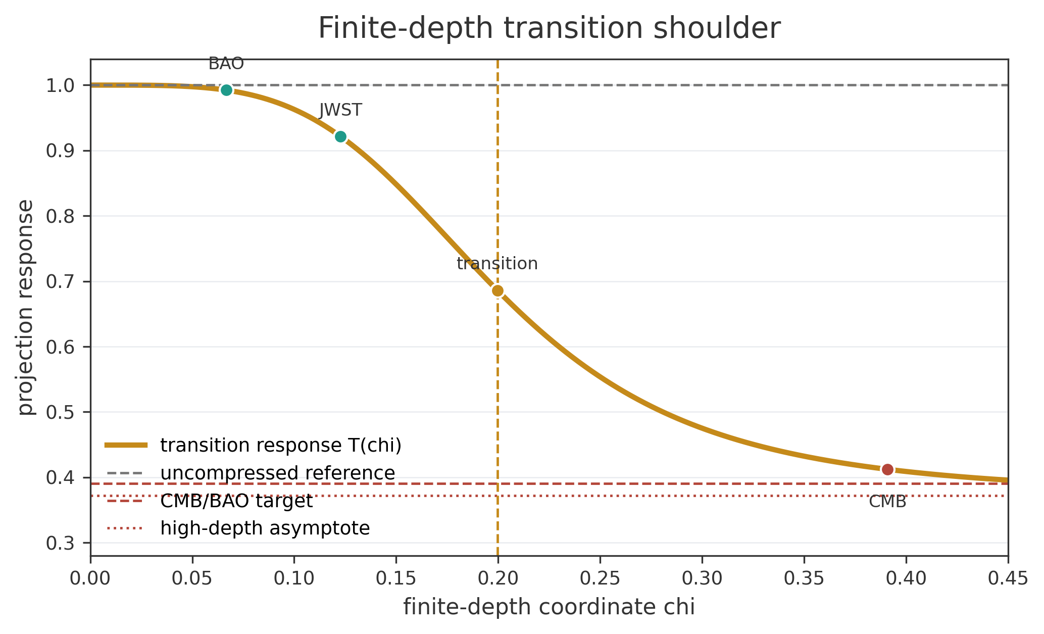
3.1 Projection Transition Displayed as \(T(\chi)\)
The transition behavior is represented in \(\chi\)-space as a compact boundary-layer recovery function:
In redshift space, the optimal recovery case employed \(\Delta = 0.627714\), \(z_t = 34.5754\), and \(m = 4\). In the \(\chi\) display, the midpoint becomes \(\chi_t = 0.1996\). This representation is useful because the transition is described as occurring at approximately one-fifth of the assumed finite-geometry depth, rather than being defined solely by a large redshift value. This is a coordinate transformation of the existing transition behavior, not a new derivation.
See the Quantitative Appendix for transition-function definitions and stage-output mapping.
3.2 JWST Mass-Size Projection Analysis
The initial galaxy analysis utilizes the Labbé et al. red massive candidate sample and the Baggen et al. structural subset. Labbé et al. identified red candidate massive galaxies at \(z \approx 7.4\)–\(9.1\), and Baggen et al. measured compact effective radii for the subset with viable structural fits. The present calculation does not refit SEDs or morphologies; rather, it evaluates how published mass and radius values shift under a simple projection conversion.
A fourth-power projection shoulder centered in the JWST redshift range is employed for sensitivity testing:
Technical note
The amplitude \(\Delta = 0.627714\) is retained from the recovery transition, while the midpoint is shifted to \(z_s = 8\). This tests a weaker high-redshift shoulder in the red massive galaxy regime rather than the main BAO-CMB transition.
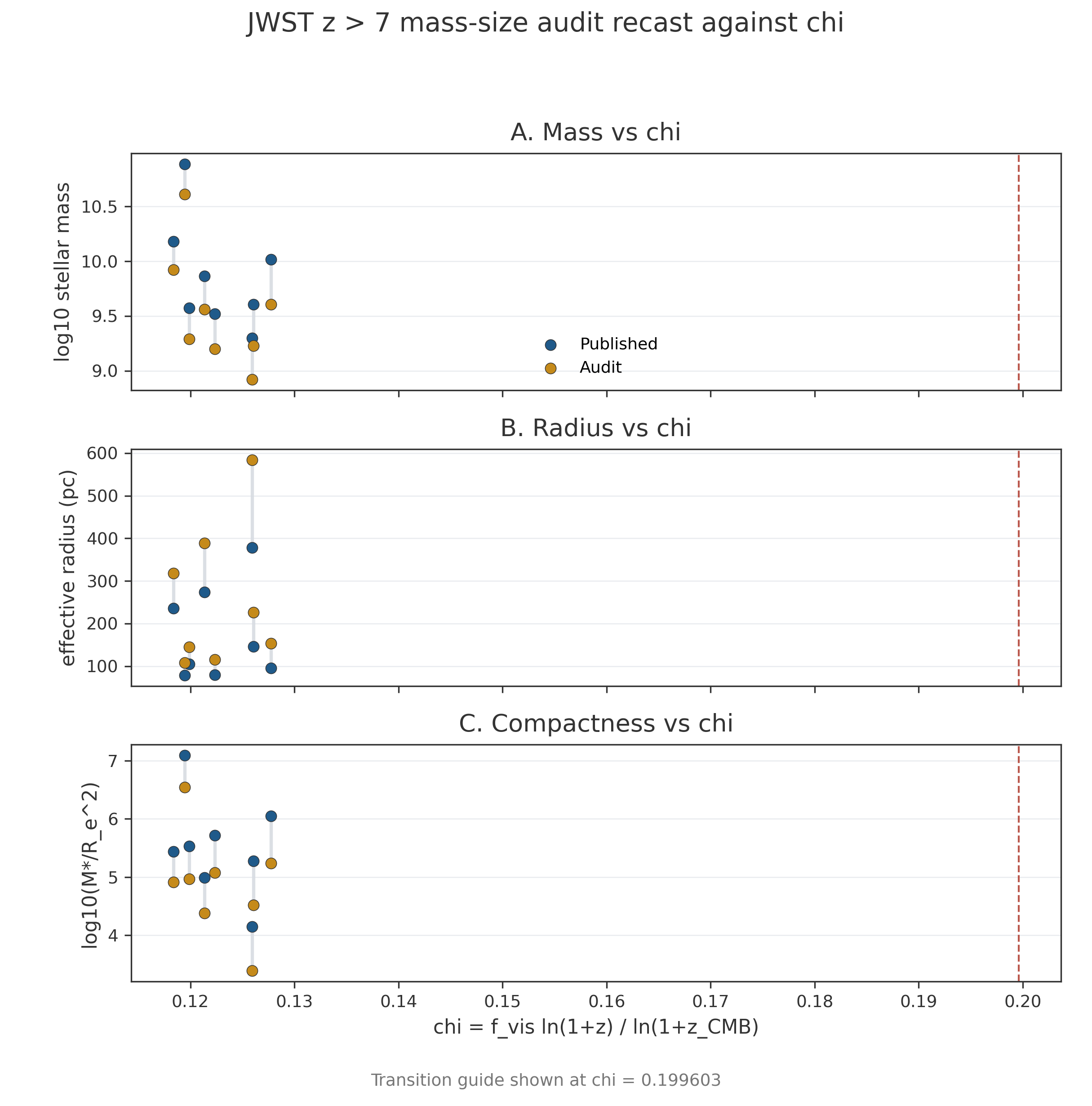
Table 2-3. Median before/after values in the \(z > 7\) mass-size projection analysis.
| Quantity | Published Median | Analysis Median | Direction |
|---|---|---|---|
| Median log stellar mass | 9.7369 | 9.4260 | Lower mass |
| Median effective radius (pc) | 125.5000 | 189.9640 | Larger size |
| Median log compactness | 5.4826 | 4.9411 | Lower compactness |
3.3 Expanded PRIMAL Spectroscopy Analysis
The expanded spectral analysis utilizes the JWST-PRIMAL catalog [47], a public JWST/NIRSpec reference sample for reionization-era galaxies. The processed sample contains 584 objects spanning \(z = 5.0\)–\(13.4\), including 134 objects at \(z \ge 7\), 51 at \(z \ge 8\), and 17 at \(z \ge 10\). The catalog provides spectroscopic redshift, UV magnitude, UV slope \(\beta_{\text{UV}}\), \([OIII]\)+H\(\beta\) equivalent width, Ly\(\alpha\) damping parameter \(D(\text{Ly}\alpha)\), O32, line fluxes, and sky position [48] [49].
Table 2-4. PRIMAL sample summary used for the expanded spectral and sky-position analysis.
| Metric | Value |
|---|---|
| Total PRIMAL rows | 584.0000 |
| Redshift min | 5.0019 |
| Redshift max | 13.3605 |
| \(z \ge 7\) count | 134.0000 |
| \(z \ge 8\) count | 51.0000 |
| \(z \ge 10\) count | 17.0000 |
| \(\beta_{\text{UV}}\) available | 584.0000 |
| \([O III]\) | 519.0000 |
| O32 positive finite | 500.0000 |
| Spectral residual model \(n\) | 473.0000 |
| Spectral-only residual \(R^2\) | 0.1243 |
3.4 Gravitational-Regime Analysis
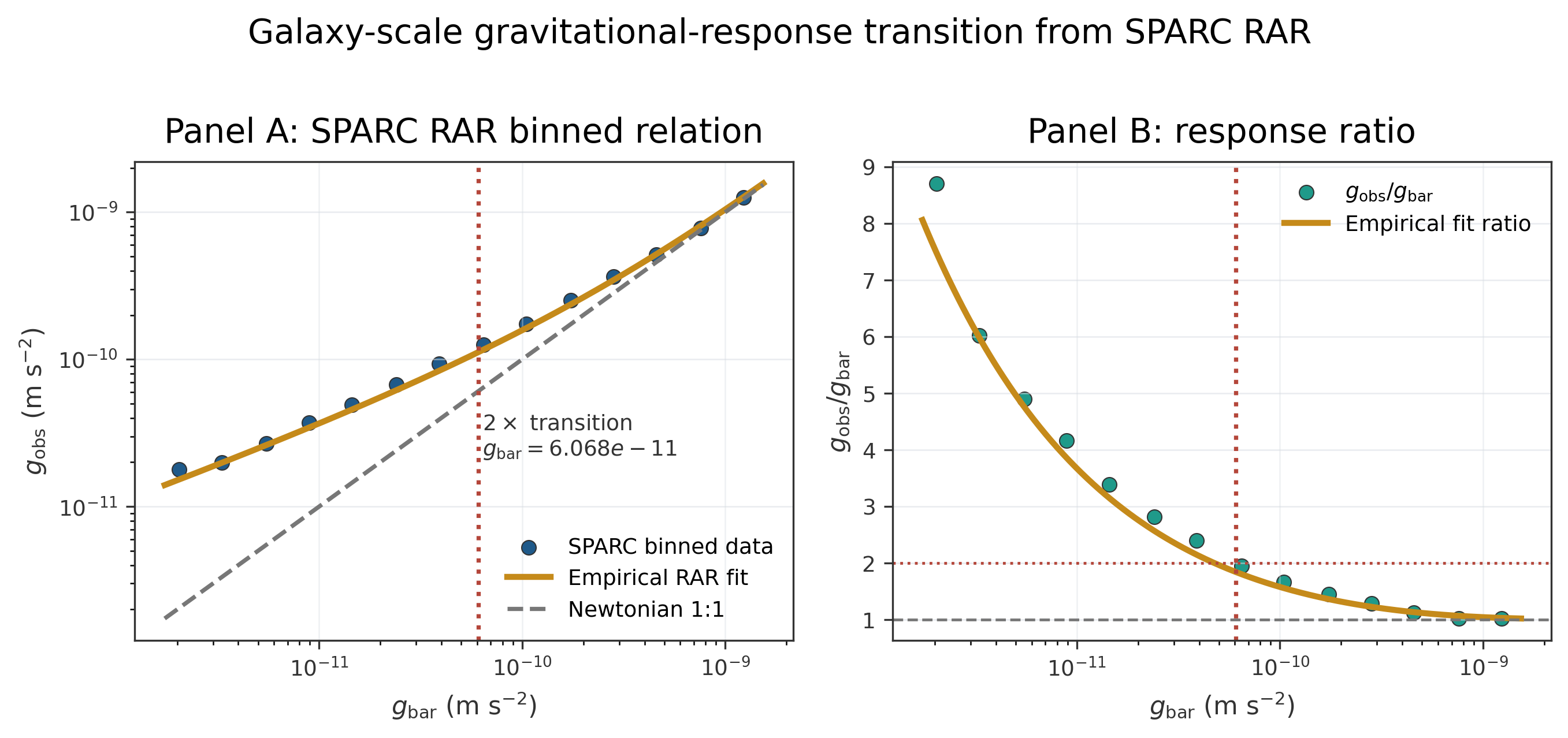
The gravitational analysis incorporates three empirical diagnostics. The galaxy-scale test utilizes the published SPARC binned radial acceleration relation, which compares the observed centripetal acceleration from rotation curves with the acceleration predicted from the observed baryonic mass distribution [50] [51]. The binned relation was fit with the empirical RAR form:
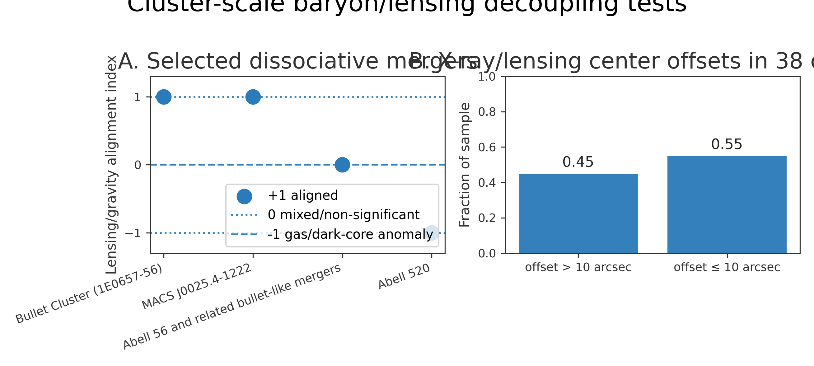
where \(g^\dagger\) is the characteristic acceleration scale. The response ratio \(g_{\text{obs}}/g_{\text{bar}}\) is then used as a dimensionless measure of gravitational-regime departure. The cluster-scale test utilizes a literature-coded set of dissociative mergers, where gravitational-lensing centers, hot X-ray gas, and galaxy concentrations are spatially separated [58]. The large-scale test utilizes published velocity-flow basin results from Laniakea and Cosmicflows-4 to evaluate whether gravitational flow domains provide a large-scale analogue of regime boundaries [52] [53].
4. Results
4.1 Regime Ordering via the \(\chi\) Coordinate
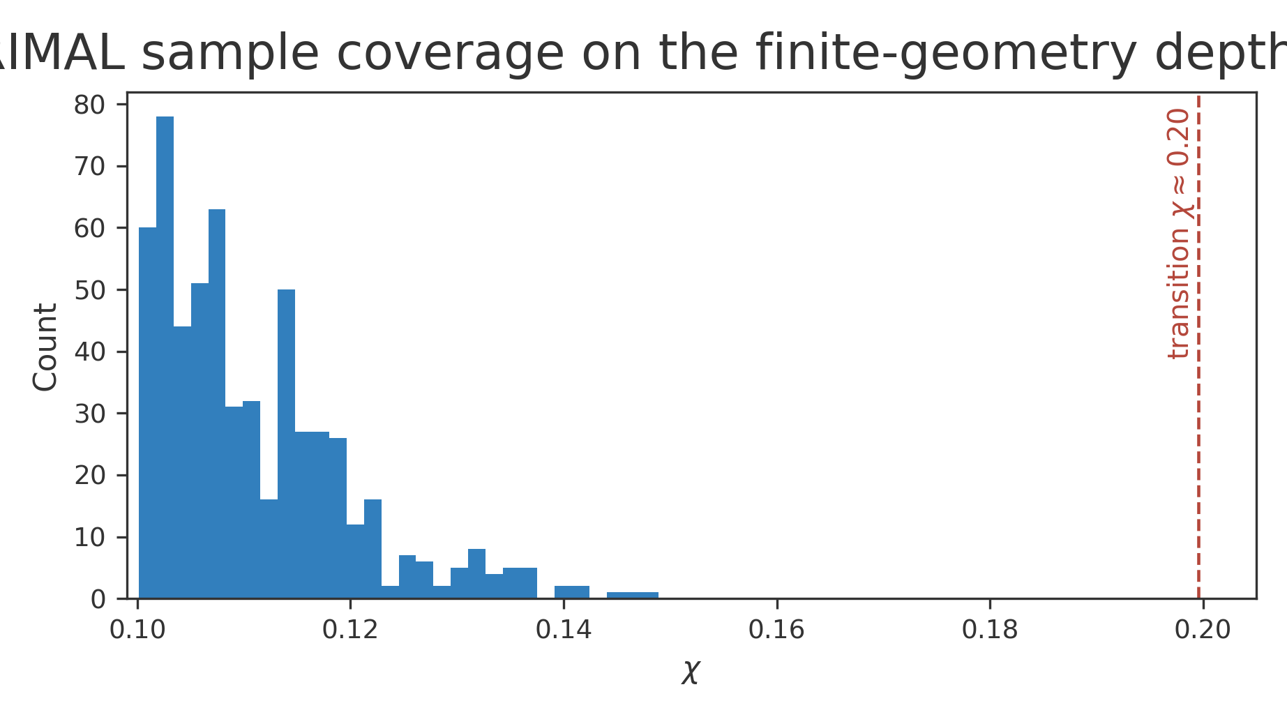
The depth coordinate organizes the primary regimes into a simple linear sequence. The BAO high end lies at \(\chi = 0.0667\). The JWST \(z \approx 8\) regime lies near \(\chi = 0.1228\), and a \(z = 14.32\) object would be positioned near \(\chi = 0.1525\). The reconstructed transition midpoint occurs at \(\chi = 0.1996\), while the CMB-side scale is at \(\chi = 0.390906\). In this ordering, JWST \(z > 7\) galaxies are not situated at the transition itself, but are positioned on the approach toward it.
4.2 Mass-Size Trends
The Labbé-Baggen analysis yields a constructive result: the median log stellar mass shifts from 9.7369 to 9.4260, the median effective radius increases from 125.5 pc to 190.0 pc, and the median compactness proxy \(\log_{10}(M_\star/R_e^2)\) decreases from 5.4826 to 4.9411. These shifts demonstrate that the projection correction acts in the direction necessary to reduce the "too-massive and too-compact" tension.
4.3 Spectral Color Residuals
The expanded PRIMAL analysis is more restrictive. Higher \(\beta_{\text{UV}}\) corresponds to a redder UV continuum; however, in the full PRIMAL sample, \(\beta_{\text{UV}}\) becomes bluer with increasing redshift. The descriptive Pearson correlation between \(\beta_{\text{UV}}\) and redshift is \(-0.226\). Correlations with spectral features indicate that conventional galaxy physics remains dominant: \(\beta_{\text{UV}}\) correlates with \(D(\text{Ly}\alpha)\), \([OIII]\)+H\(\beta\) equivalent width, and O32. A regression against \(M_{\text{UV}}\), \(\log EW([OIII]+\text{H}\beta)\), \(D(\text{Ly}\alpha)\), and \(\log O32\) explains a modest fraction of the \(\beta_{\text{UV}}\) variance (\(R^2 = 0.124\)). The residual \(\beta_{\text{UV}}\) trend against \(\chi\) remains weak.
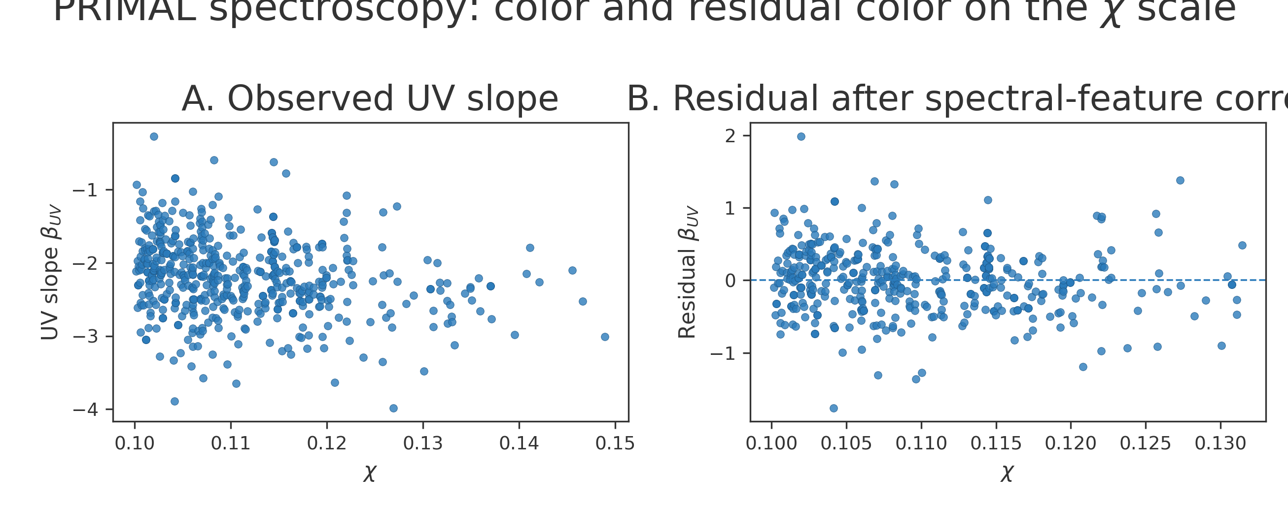
Table 2-5. Descriptive correlations from the PRIMAL spectral and sky-position analysis.
| Test | \(n\) | Pearson \(r\) |
|---|---|---|
| \(\beta_{\text{UV}}\) redness vs \(z\) | 584 | -0.2258 |
| \(\beta_{\text{UV}}\) redness vs \(D(\text{Ly}\alpha)\) | 584 | -0.1633 |
| \(\beta_{\text{UV}}\) redness vs \(\log EW([O III])\) | 519 | -0.1969 |
| \(\beta_{\text{UV}}\) redness vs \(\log O32\) | 500 | -0.2778 |
| \(\log O32\) vs \(z\) | 500 | 0.3288 |
| \(z\) vs RA | 584 | -0.0612 |
| \(z\) vs Dec | 584 | -0.0741 |
| Spectral residual \(\beta_{\text{UV}}\) vs \(z\) | 473 | -0.1058 |
| Spectral residual \(\beta_{\text{UV}}\) vs RA | 473 | 0.0654 |
| Spectral residual \(\beta_{\text{UV}}\) vs Dec | 473 | 0.0690 |
| Residual \(\beta_{\text{UV}}\) (no \(z\) in model) vs \(\chi\) | 473 | -0.1099 |
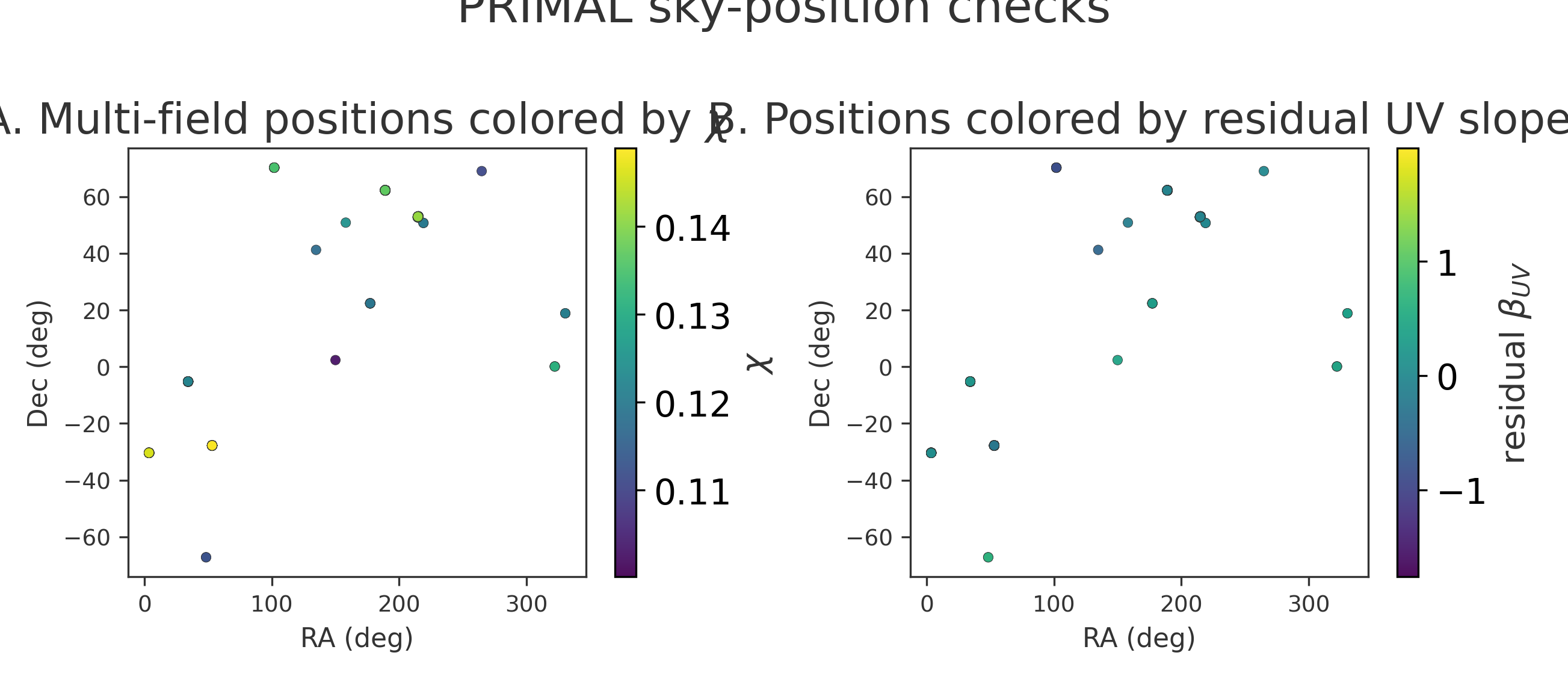
4.4 Sky-Position Distribution
Sky-position tests similarly yield limited results. In the PRIMAL sample, redshift shows little linear dependence on RA or Dec (\(r = -0.061\) for \(z\) vs RA; \(r = -0.074\) for \(z\) vs Dec). The residual \(\beta_{\text{UV}}\) field is also weakly correlated with sky position. While these results do not rule out a geometric interpretation—given that the public sample is assembled from multiple programs with differing selection functions—they indicate that the current data do not exhibit a simple RA/Dec phase-boundary pattern.
4.5 Gravitational-Regime Tests
The gravitational tests serve as a bridge from projection-depth behavior to local and large-scale gravitational response. They evaluate whether gravitational observables contain natural transition scales or domain boundaries comparable to the finite-geometry language developed in this work.
Table 2-6. Gravitational-regime analysis summary.
| Test | Scale | Key Result | Status |
|---|---|---|---|
| SPARC RAR | Galaxy | \(g^\dagger = 9.89 \times 10^{-11}\) m s\(^{-2}\); 2\(\times\) response at \(6.07 \times 10^{-11}\) m s\(^{-2}\) | Strongest transition |
| Dissociative clusters | Cluster | Mixed offsets; 45% of 38 clusters have X-ray/lensing offsets \(> 10''\) | Informative but ambiguous |
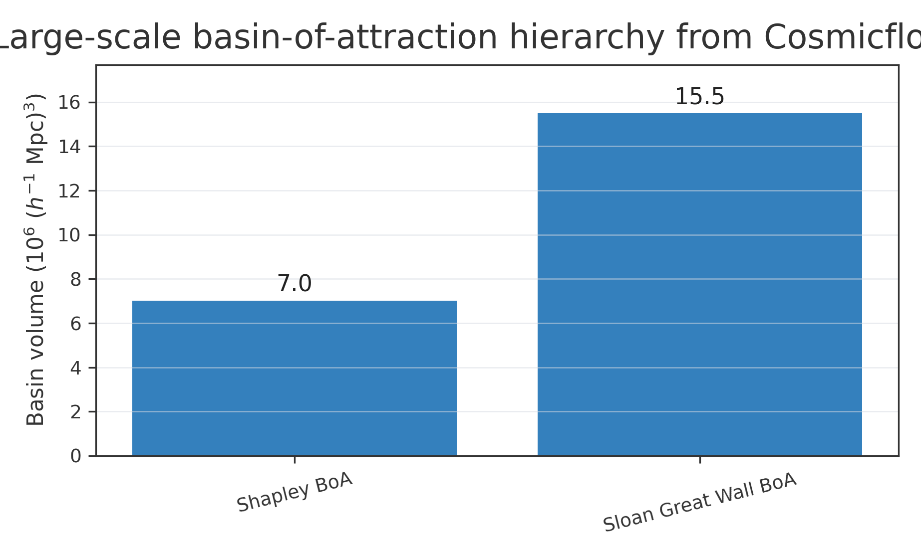
| Attractor basins | Large scale | Laniakea, Shapley, and Sloan Great Wall velocity-flow basins | Conceptual analogue |
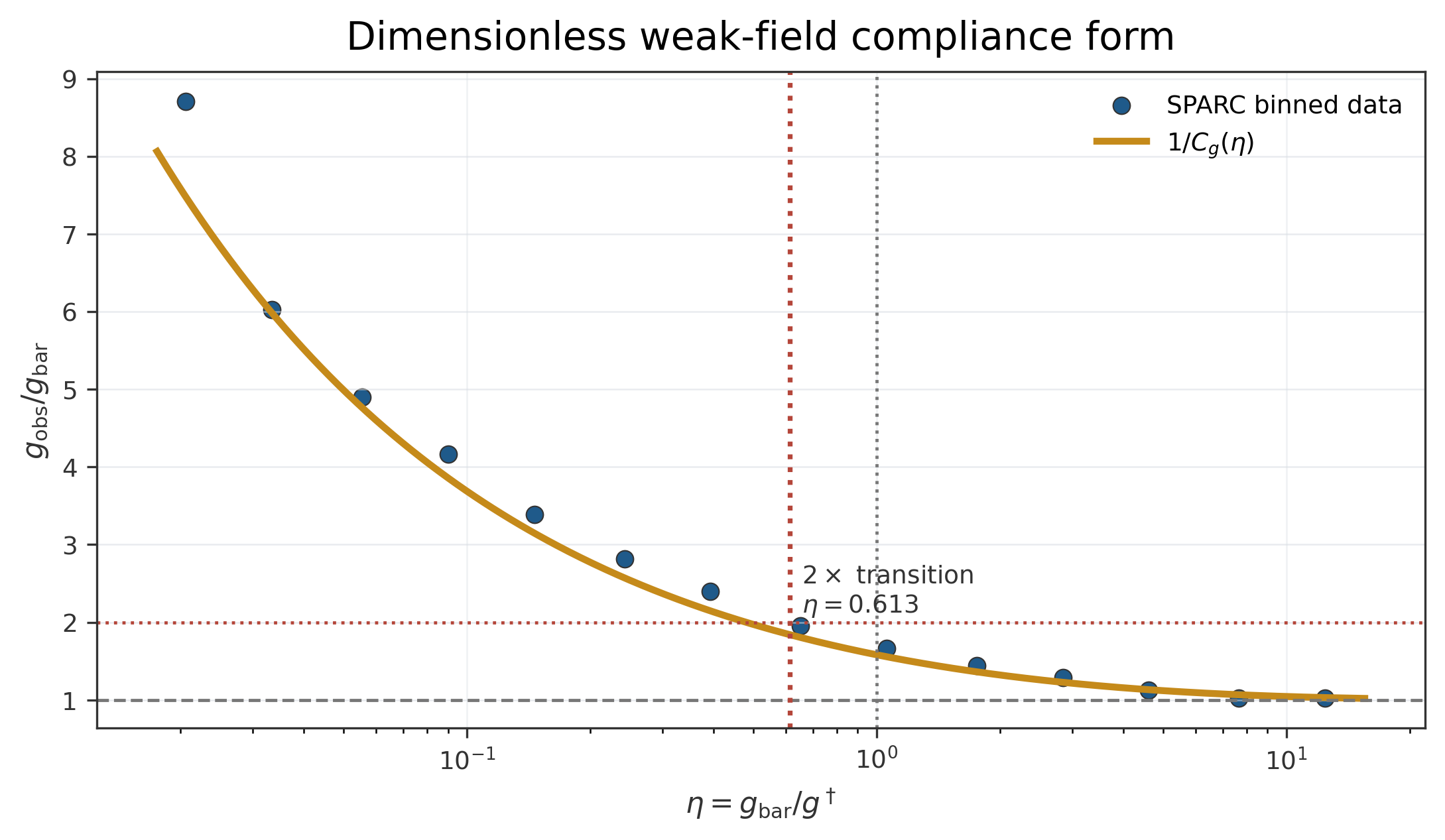
The galaxy acceleration test yields the most definitive result. The SPARC binned radial acceleration relation is fit by Equation (2-8) with \(g^\dagger = 9.89 \times 10^{-11}\) m s\(^{-2}\). The observed-to-baryonic response reaches approximately a factor of two at \(g_{\text{bar}} = 6.07 \times 10^{-11}\) m s\(^{-2}\). Above this characteristic scale, the relation approaches the Newtonian one-to-one baryonic prediction. Below it, the observed gravitational response increasingly exceeds the baryonic prediction (Figure 2-7). This constitutes a clear gravitational-regime transition expressed as a dimensionless response ratio.
The dissociative-cluster test is informative but less definitive. The Bullet Cluster and MACS J0025.4-1222 exhibit lensing/gravity peaks separated from the hot X-ray gas and aligned more closely with the collisionless component [54] [55]. Abell 520 serves as a counterexample, featuring a dark-core morphology associated with the X-ray gas and a relative lack of bright galaxies [56] [57]. In a sample of 38 clusters, 45 percent exhibited projected offsets larger than 10 arcseconds [59]. These results demonstrate that baryonic gas and gravitational lensing centers can decouple, though they do not independently distinguish finite-geometry response from collisionless dark matter (Figure 2-8).
The attractor test is best interpreted as a conceptual large-scale analogue. Laniakea is defined via velocity-flow watersheds, with galaxy motions organized into an inward-flowing basin after subtracting mean expansion and long-range flows [52]. Cosmicflows-4 research suggests that Laniakea may be part of the larger Shapley basin, with the Sloan Great Wall basin recovered as the largest in that analysis [53]. These results support the conceptual framework of gravitational domains and watershed boundaries, though they remain model-dependent as they rely on peculiar-velocity reconstructions (Figure 2-9).
4.6 Matter-Void Foam Morphology and Finite-Response Screening
The projection-depth, spectroscopic-residual, and gravitational-response tests are extended to matter-void morphology. This screen evaluates whether the large-scale distribution of void space and web-bounded foam structure is better organized by the full finite-response coordinate than by redshift ordering alone.
The analysis utilizes the public SDSS DR7 VAST void catalogs, which provide complementary void populations identified via VoidFinder and V2 watershed methods [60]. The Planck 2018 VAST release reports 1163 VoidFinder voids, 531 V2/VIDE voids, and 518 V2/REVOLVER voids in the SDSS DR7 main-survey volume to \(z = 0.114\), with effective radii and centers provided in the ASCII catalogs [61] [62]. While this depth is insufficient to sample the transition range, it allows for an evaluation of how different void definitions respond to the finite-geometry coordinate.
Technical note
Because the catalog reaches only \(z = 0.114\), it probes the early side of the response curve. It serves as an early-range morphology screen for \(D = AG\), rather than a direct sample of the deeper transition region.
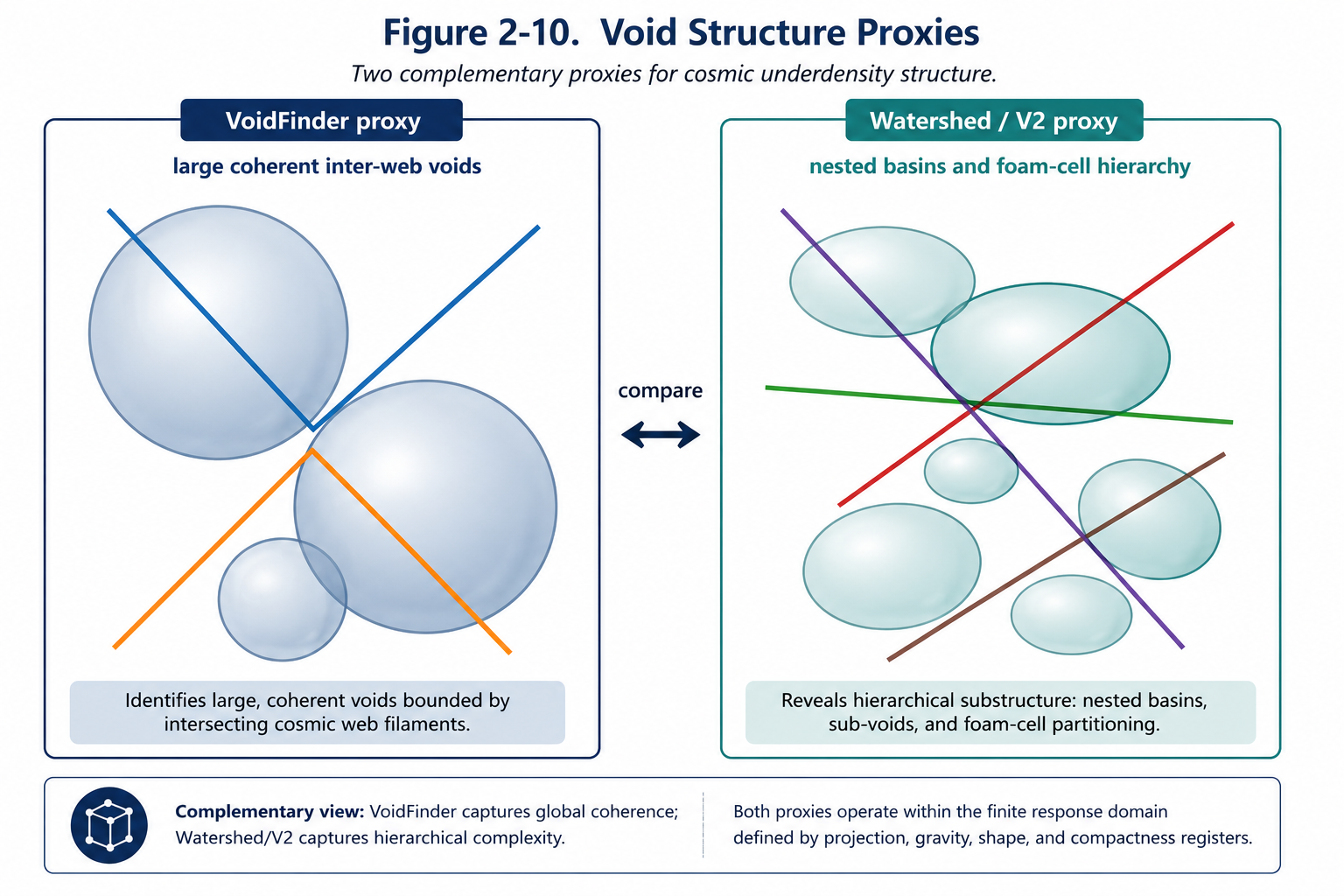
VoidFinder and watershed methods are treated as complementary shape filters. VoidFinder acts as a proxy for large coherent inter-web void regions, while VIDE and REVOLVER serve as proxies for nested basin-like void structure within the foam. Watershed algorithms segment the density field into basins and preserve hierarchical structure, while VIDE utilizes Voronoi tessellation and a ZOBOV-based watershed transform to construct void catalogs [63] [64] [65]. Differences among these definitions produce measurable morphology signals.
Previous morphology screens compared standard redshift \(z\) with the accumulated finite-geometry coordinate:
That analysis was incomplete as it omitted the response-weakening term used in the finite deformable-geometry model. The present screen therefore compares void metrics against four predictors:
When \(D\) is used as a response-function argument, it is normalized as \(D_n = D/D_0\), where \(D_0\) is a reference response scale with the same units as \(D\). The raw \(D\) is retained for the morphology screen.
See the Quantitative Appendix for \(D_n\) normalization and response-function bookkeeping.
Technical note
For comparison with the projection transition, the same redshift bins can be expressed as \(X = A/A_t\). This \(X\) coordinate identifies where a sample lies relative to the recovery transition and complements the \(z, A, G,\) and \(D\) predictor comparison.
For this initial catalog-level test, \(d\) is treated as a normalized redshift-distance proxy, \(d_{\text{norm}} = z / z_{\text{max}}\), and \(g_0\) is set to 1. The response scale \(d_b\) is scanned across values of 0.05, 0.10, 0.20, 0.30, 0.50, and 1.00. This normalization ensures the screen remains dimensionless and reproducible.
A foam index is defined as the ratio of watershed-defined voids to large VoidFinder voids within the same redshift or response-coordinate bin:
The tested morphology vector is thus expressed as:
where \(I_{\text{foam}}\) is the foam-index proxy, \(R_{\text{eff}}\) is the effective radius, \(V_e\) is void ellipticity, and \(C_{\text{shape}}\) is a hierarchy/connectivity proxy. Dimensional vector entries are standardized before comparison. Each metric is compared against \(z, A, G,\) and \(D\) using linear, quadratic, and two-segment piecewise fits, with labels assigned based on \(R^2\), RMSE, monotonicity, and Spearman trend diagnostics.
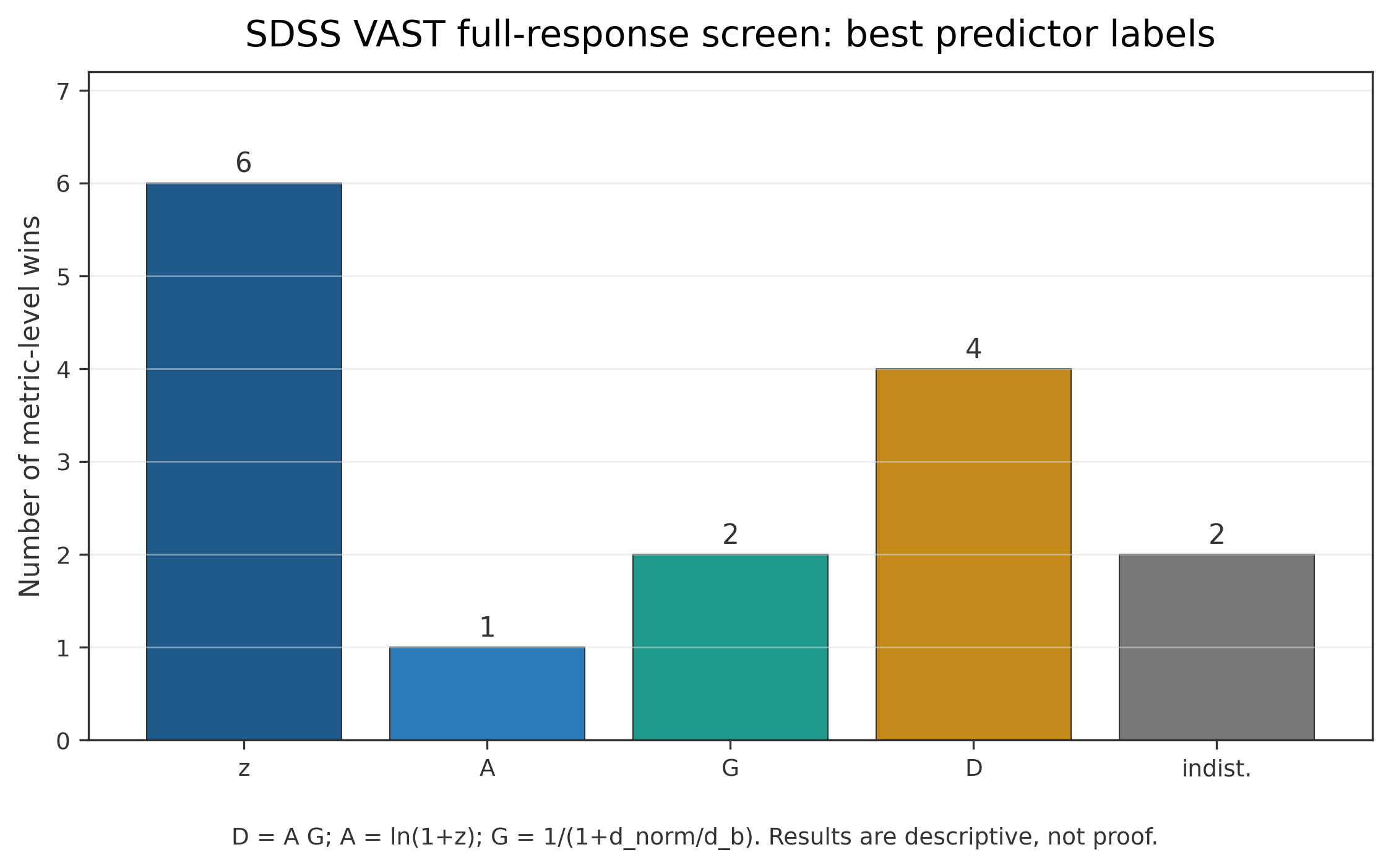
Table 2-7. Summary of the SDSS VAST full finite-response morphology screen.
| Predictor Label | Metric-Level Wins | Representative Metrics | Interpretation |
|---|---|---|---|
| D better | 4 | REVOLVER foam index; REVOLVER mean ellipticity; VIDE mean ellipticity; VoidFinder median radius | Several independent shape metrics are better organized by the full response variable. |
| G better | 2 | VoidFinder count; VoidFinder mean ellipticity | Some metrics respond most strongly to the weakening function alone. |
| A better | 1 | VIDE count | Accumulated deformation alone is not the dominant predictor. |
| z better | 6 | REVOLVER count; VIDE foam index; mean foam index; selected median ellipticity and radius metrics | Standard redshift remains competitive and frequently superior. |
| Indistinguishable | 2 | VIDE median ellipticity; VIDE median radius | Some metrics cannot separate predictors within the SDSS redshift range. |
The critical outcome is the distribution of winning labels. \(D = AG\) performs better than \(A\) alone for several independent morphology metrics, including the REVOLVER foam index and mean ellipticity in both REVOLVER and VIDE. This indicates that the response-weakening term \(G\) helps organize shape quantities that are not clarified by accumulated deformation \(A\) alone. The optimal response-scale value in the tested grid is \(d_b = 1.0\), suggesting that the preferred response weakening is gradual across the SDSS range. A sharply decaying response function is not favored by this early-range morphology screen.
Standard redshift remains the best predictor for several metrics, including the mean foam index and selected radius and ellipticity summaries. Consequently, while the full finite-response variable warrants testing in deeper object-level surveys [66], the shallow SDSS screen remains subordinate to the stronger JWST and SPARC constraints.
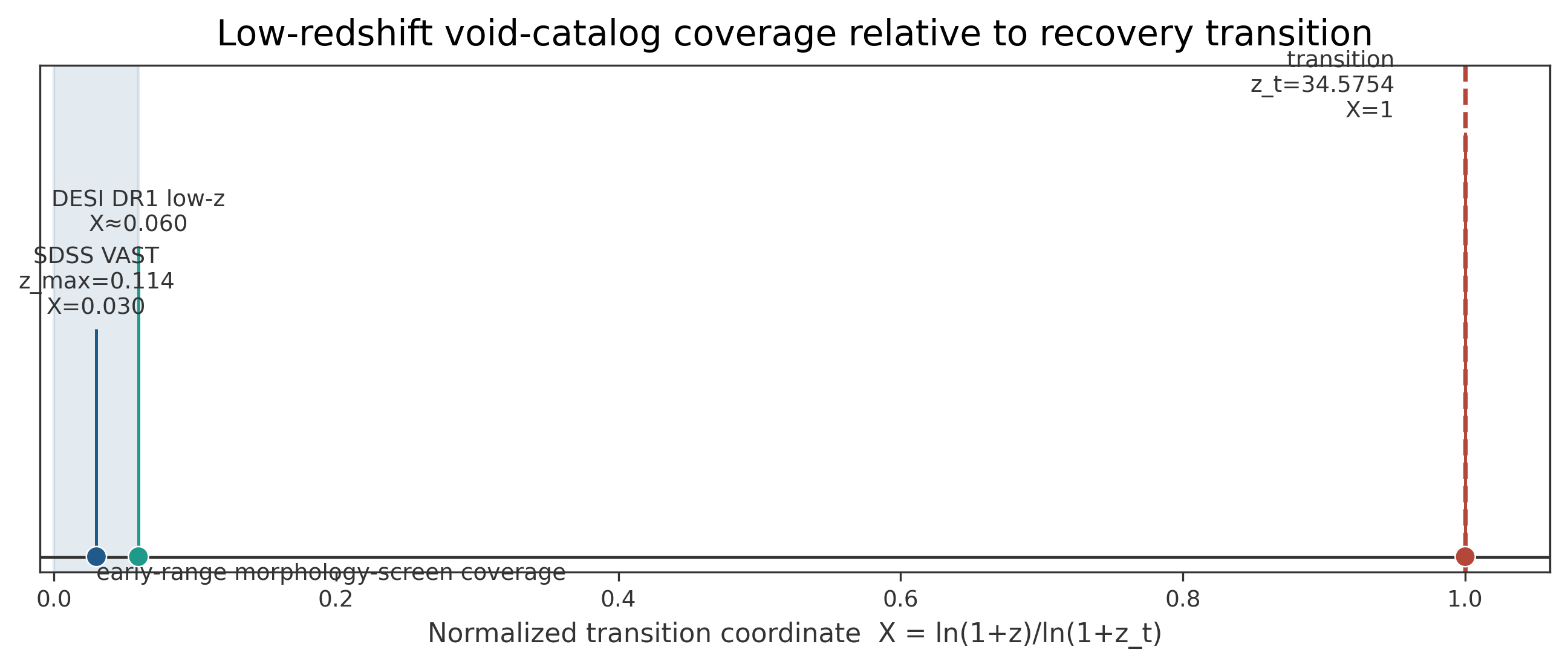
The relevant transition is the recovery transition recast as \(\chi \approx 0.20\), or equivalently \(X = 1\). This transition corresponds to \(z_t = 34.5754\) and \(A_t = \ln(1+z_t) \approx 3.572\). Since the SDSS screen samples only \(X \approx 0.03\), it serves as an early-range morphology screen for the \(D = AG\) variable rather than a direct pressure-transition test. A decisive shape test would require a significantly deeper structure probe.
5. Discussion
Three classes of observational registers are compared. The JWST sections evaluate projection conversion using derived galaxy properties while holding direct observables, such as redshift and flux, as close to measurement as possible. The gravity sections recast acceleration and compactness behavior as finite-response regimes. The foam-shape and black-hole sections define shape and boundary targets. The relative weight of these results varies: the JWST mass-size conversion and the SPARC transition serve as current constraints, while matter-void and compactness results are early-stage constraints and model targets.
5.1 Strengths of the Model
The strongest evidence is the mass-size direction of effect. Under the projection shoulder, published high-redshift galaxies become less massive, larger, and less compact. This aligns with the requirements to resolve early-galaxy tension if part of the issue stems from the expansion-based conversion between redshift, luminosity distance, angular-size distance, and physical age. The precision of the chosen shoulder is less critical than the fact that raw redshift, flux, and angular size can be held fixed while derived masses and sizes are recomputed under an alternative projection law.
Because the PRIMAL color and sky-position analyses do not provide independent support, the primary JWST leverage remains in the mass-size conversion test.
5.2 Spectral and Void-Shape Constraints
The PRIMAL results constrain the projection interpretation. UV color and sky position do not provide independent support for a finite-geometry boundary. Factors such as strong rest-optical emission lines, ionization state, and dust all influence high-redshift galaxy appearance. The expanded sample trends bluer with redshift, and the residual color signal after spectral-feature correction remains weak. A geometric interpretation is therefore more effectively tested through mass-size-age conversion.
The void-shape screen is primarily constrained by depth. Its value is methodological, demonstrating how to formulate a deeper matter-void shape test against \(z, A, G,\) and \(D\). It does not displace the stronger constraints set by the JWST mass-size conversion and the SPARC transition.
5.3 Required Projection-Conversion Tests
A robust projection-conversion test requires spectroscopic redshifts and line diagnostics from PRIMAL or the DAWN JWST Archive, homogeneous morphology and size measurements, and a controlled projection conversion applied to luminosity and angular-size distance separately. The decisive question is whether finite-geometry conversion reduces the mass-size-age tension without degrading direct spectroscopic observables. If this effect persists across multiple fields and independent reduction pipelines, it constitutes a strong test of projection-regime physics.
5.4 Gravitational-Regime Implications
The gravitational analysis strengthens the finite-geometry program by identifying the SPARC acceleration transition. This result shows a repeatable, dimensionless departure in gravitational response near \(10^{-10}\) m s\(^{-2}\), independent of the redshift-depth coordinate. This serves as a natural gravity analogue of a regime boundary, where baryons remain the local source term but the effective gravitational response shifts below a characteristic scale.
The cluster and attractor tests are informative but less decisive. Dissociative clusters show that lensing response and hot gas can occupy different observational registers during mergers, but collisionless dark matter already accounts for much of this behavior in the standard framework. Velocity-flow basins, such as Laniakea and the Shapley basin, provide a suggestive large-scale vocabulary of gravitational domains, though these reconstructions are model-dependent (Figure 2-9).
5.5 Finite-Geometry Correction for the GR Limit
The gravitational results suggest a conservative route for connecting the model to relativistic gravity. The local success of General Relativity is retained, and the finite-deformable framework is expressed as an effective correction that becomes negligible in high-acceleration, weak-boundary regimes, activating only when a system crosses a deformation threshold:
Here, \(F_{\mu\nu}\) represents an effective finite-geometry response term rather than a new matter component. This term must vanish where GR tests are successful and must be constrained by conservation requirements. A phenomenological decomposition is given as:
In this notation, \(B_{\mu\nu}\) sets the direction and structure of the correction, \(\alpha\) sets its amplitude, and \(C\) is a dimensionless compliance function. The regime variables are defined as:
These variables describe different boundary approaches: \(\eta\) for the galaxy acceleration regime, \(u\) for the Schwarzschild compactness measure, and \(D_n\) for the normalized morphology-response coordinate. The SPARC result provides the first empirical calibration, where the binned relation is described by a dimensionless compliance factor:
Equation (2-18) recasts the radial acceleration relation as a weak-field finite-geometry compliance law. At \(\eta \gg 1\), the response ratio approaches unity and baryonic gravity is recovered. At \(\eta\) below order unity, the geometry behaves as more compliant, and the observed response exceeds the baryonic prediction. This interpretation relates empirically to MOND and relativistic MOND-like theories, although the present model treats the transition as a finite-geometry regime effect [67] [68] [69].
This weak-field comparison sits alongside MOND and relativistic-MOND review literature, though it utilizes SPARC/RAR behavior as a finite-geometry compliance register rather than a direct adoption of MOND dynamics [81].
See the Quantitative Appendix for response-function notation used by the register bridge.
5.6 Black Holes as Compactness-Boundary Tests
The black-hole compactness register establishes a boundary-condition target, defining what a finite-deformable model must satisfy at the compactness limit while remaining consistent with the \(\chi\), JWST, SPARC, and void-shape results.
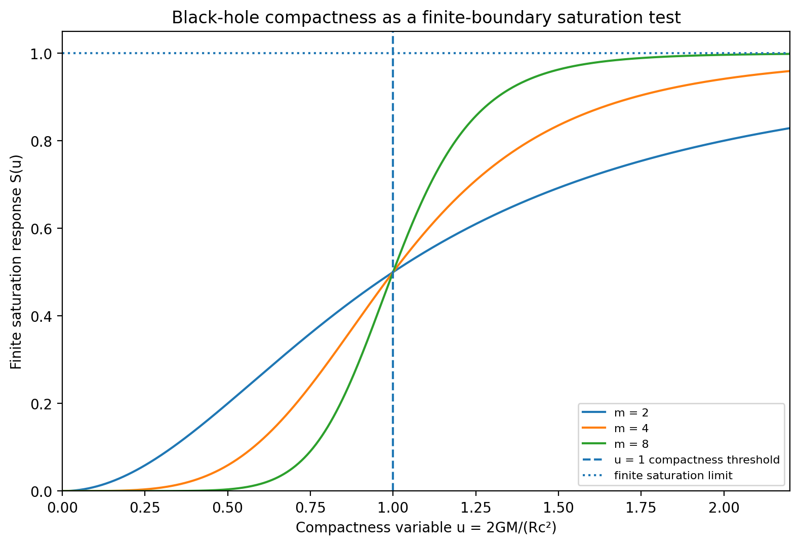
The black-hole case extends the analysis to the strongest compactness limit. The dimensionless variable \(u = 2GM/(Rc^2)\) compares a system's Schwarzschild radius with the radius at which the mass is evaluated. For a nonrotating exterior solution, \(u = 1\) marks the horizon scale. In the finite-deformable framework, the horizon is not treated as a physical infinity but as the entry into a compactness regime where the relationships between mass, time, distance, and curvature are no longer described by extending ordinary exterior coordinates without limit.
A finite-saturation target is defined as:
Here, \(S(u)\) is a compactness-response function, \(u_c\) is the order-unity threshold, and \(m\) controls transition sharpness. The function remains small in weak compactness, rises rapidly near the horizon-scale threshold for large \(m\), and approaches a finite value instead of diverging. This defines a boundary condition: preserve the exterior behavior that makes GR successful while replacing the singular endpoint with a finite interior response. This framing aligns with regular or nonsingular black-hole programs that seek finite interior geometries [1] [2] [70].
The schematic black-hole contribution to the finite-geometry term is written as:
In this expression, \(\alpha_{\text{BH}}\) sets the amplitude of the compactness-regime correction, \(B_{\mu\nu}(\text{BH})\) defines its tensor structure, and \(S(u)\) controls its activation. A future theory would derive this term from an action or another conservation-compatible principle, recovering the exterior Schwarzschild/Kerr behavior tested by black-hole shadows and gravitational-wave mergers while modifying only the interior or near-boundary extrapolation [71] [72].
Such an extension would also need to demonstrate that any \(S(u)\)-driven interior modification leaves exterior lensing, ringdown, and shadow observables unchanged to current precision.
5.7 Shape-Test Implications and Pressure-Transition Target
The matter-void morphology screen adds a shape register to the projection and gravity registers. High-redshift galaxy sections evaluate whether derived properties are altered by projection-depth conversion, and gravity sections evaluate whether acceleration and compactness regimes can be written as finite-response boundaries. The void test asks whether underdense space and web-bounded foam structure organize under the finite deformable response variable.
The SDSS VAST catalogs demonstrate that this is a measurable question, and the full response coordinate \(D = AG\) improves several independent shape metrics relative to \(A\) alone. While standard \(z\) remains the strongest predictor for other metrics, the available SDSS redshift range only samples the earliest part of the normalized transition coordinate.
The pressure question follows the shape test. In the present framework, the pressure-transition target corresponds to the \(\chi \approx 0.20 / X = 1\) recovery regime. A physical test would evaluate whether matter-coupled deformation response weakens toward a vacuum-like state as \(X\) approaches 1. The pressure-like quantity would decrease from positive response toward a near-zero vacuum response, rather than crossing into a negative-pressure regime. The current SDSS test is unable to reach that regime, serving only as an early-range morphology screen for the \(D = AG\) variable.
6. Limitations
The present analysis utilizes processed catalog products and descriptive correlations. The Labbé-Baggen mass-size sample is limited in size. The PRIMAL sample is more extensive but is not a uniform all-sky survey, and field selection remains a relevant factor. The residual-color regression employs a compact model and does not include full hierarchical treatment. Full SED refitting, morphology remeasurement, covariance propagation, and AGN removal are outside the scope of this pass.
The \(\chi\) coordinate depends on \(f_{\mathrm{vis}} = 0.390906\) as the organizing scale. The SPARC result is based on binned acceleration data, the cluster comparison uses a literature-coded merger set, and the attractor analysis depends on peculiar-velocity reconstructions built on a background cosmological model. The finite-geometry correction term is phenomenological, and the black-hole saturation function is specified as a boundary target. A comprehensive relativistic theory would need to define \(F_{\mu\nu}\) from an action or other dynamical principle and demonstrate compatibility with the Bianchi identity, energy-momentum conservation, gravitational lensing, Solar System tests, and black-hole observations. Finally, the SDSS DR7 VAST foam screen utilizes a normalized distance proxy \(d_{\text{norm}} = z/z_{\text{max}}\) and reaches only \(A = \ln(1+z) \approx 0.108\) (\(X \approx 0.030\)), meaning it does not sample the \(\chi \approx 0.20 / X = 1\) pressure-to-vacuum regime directly.
7. Conclusions
Empirical Findings
• Interpreting the separate-scale ratio 0.390906 as a finite-geometry depth scale provides a useful unitless coordinate, \(\chi\).
• Within the \(\chi\) coordinate, BAO is located near 0.067, JWST \(z \approx 8\) galaxies near 0.123, the reconstructed projection transition near 0.200, and the CMB-side scale at 0.391.
• The JWST mass-size analysis shifts derived galaxy properties in the expected direction: lower stellar mass, larger radius, and lower compactness.
• Expanded PRIMAL spectroscopy does not isolate a clean residual color or sky-position signal after spectral-feature effects are considered. The primary JWST leverage remains in mass-size conversion.
• The gravitational extension identifies the SPARC radial acceleration relation as the most definitive gravitational-regime transition, with \(g^\dagger\) near \(10^{-10}\) m s\(^{-2}\) and a 2\(\times\) response near \(6.07 \times 10^{-11}\) m s\(^{-2}\).
Technical note
• The SPARC acceleration transition can be written as a weak-field compliance law, \(g_{\text{obs}}/g_{\text{bar}} = 1/C_g(\eta)\), where \(\eta = g_{\text{bar}}/g^\dagger\) and \(C_g(\eta) = 1 - \exp(-\sqrt{\eta})\).
• The SDSS VAST matter-void screen treats the cosmic web as a foam-like architecture, using VoidFinder as a proxy for large coherent inter-web voids and V2/VIDE and V2/REVOLVER as proxies for watershed-defined basin structure.
• The full finite-response coordinate \(D = AG\) outperforms \(A\) alone for several independent shape metrics, including the REVOLVER foam index, VIDE and REVOLVER mean ellipticity, and VoidFinder median radius. However, standard \(z\) remains superior for several other metrics.
Conceptual Targets
• Dissociative clusters and large-scale basins exhibit baryon/lensing and velocity-flow decoupling, though these tests remain dynamically complex and model-dependent.
• A conservative field-equation bridge is feasible: retain General Relativity as the local high-acceleration limit and introduce an effective finite-geometry term \(F_{\mu\nu}\) that activates only near regime thresholds.
• The SDSS VAST screen reaches only \(A \approx 0.108\) (\(X \approx 0.030\)) relative to the recovery transition. The \(\chi \approx 0.20 / X = 1\) pressure-to-vacuum target therefore requires a deeper structure probe evaluated as a shape-transition test.
• Comprehensive gravity testing requires a full SPARC galaxy-by-galaxy finite-compliance fit, followed by a homogeneous cluster-offset catalog and controlled attractor-basin analysis.
Technical note
• Black holes are treated as a compactness-boundary target. The model employs \(u = 2GM/(Rc^2)\) as a compactness-regime variable and seeks finite saturation \(S(u)\), replacing the mathematical singularity with a physical boundary.
• The black-hole extension must maintain exterior GR behavior, ensure compatibility with black-hole shadows and gravitational-wave mergers, and provide finite behavior as compactness crosses the horizon-scale regime.