Chapter 1

Chapter 1: Redshift as Path Response in a Finite Deformable Geometry

Chapter 1 figure anchors

Figure 1-1 Figure 1-2 Figure 1-3 Figure 1-4 Figure 1-5 Figure 1-6 Figure 1-7 Figure 1-8 Figure 1-9 Figure 1-10 Figure 1-11 Figure 1-12 Figure 1-13

Abstract

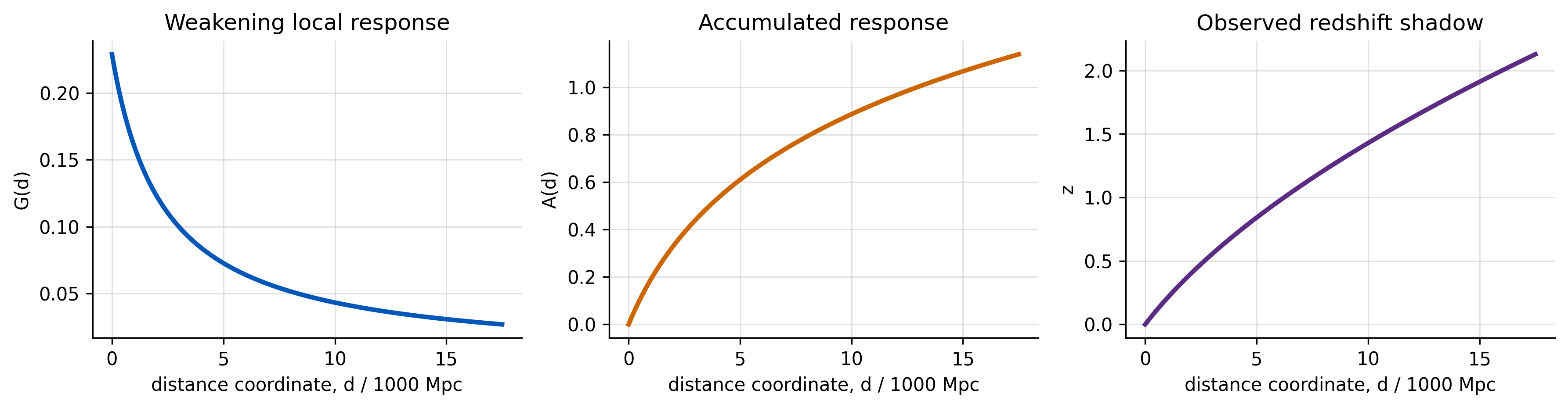
This chapter evaluates a finite deformable geometry model for redshift and distance within a non-expanding framework. In this framework, mathematical infinities are treated as limiting operations rather than physical realities. Observed redshift is modeled as an accumulated path response, \(A(d) = \ln(1 + z)\), and evaluated using the local-response law \(G(d) = g_0/(1 + d/d_b)\).

Using data from Type Ia supernovae, BAO measurements, cosmic chronometers, time-dilation constraints, and compressed CMB distance priors, the supernova-centered relation reproduces nonlinear redshift-distance curvature and remains stable across model-selection and sky-sector checks. An Alcock-Paczynski-style BAO anisotropy check using the radial-to-angular ratio \(\Delta z/\theta\) yields \(Q_{norm}(z) \approx 1.005z + 0.843\). While this scale-free BAO shape aligns with the power-law scaling of supernovae, the model breaks sharply when BAO and CMB constraints are forced to share a single sound-horizon calibration.

This failure establishes a numerical recovery target: while the BAO redshift range remains nearly unchanged, high-redshift projections must change rapidly. The optimal target identified is \(z_t \approx 34.6\), employing a fourth-power transition form with a high-redshift limit in the CMB-side compression band. The result is a repeatable supernova-scale pattern and a specific boundary-layer transition that any viable physical mechanism must explain.

These calculations assume a pre-existing, measurable universe-state; they do not describe a "before-time" event. The goal is to determine if measured redshift can be interpreted as a path response inside a finite geometry rather than as a direct measure of a universal expansion scale.

Reader note: Distant light arrives with its color shifted. This chapter asks whether that shift can be read as something that builds up over the light's journey, then checks the idea against several cosmic ruler tests. The strongest tension appears when the nearer galaxy-clustering ruler and the oldest-light ruler are forced to use one shared scale.

Introduction

The model operates on the principle that mathematical infinities require observational support before they are treated as physical structures. In General Relativity, singularity theorems suggest that classical spacetime can become geodesically incomplete [1] [2] [3]. This model treats such incompleteness as a signal that a description has reached the edge of its domain, rather than as evidence of physically realized infinite density or curvature. Similarly, quantum mechanics suggests that physically meaningful states must yield finite, normalizable probabilities, while ideal plane waves are treated as mathematical generalizations rather than finite-energy physical objects [4] [5].

This logic motivates a cosmology that does not assume infinite extent. Finite and multiply connected cosmologies have a substantial history, with research showing that local curvature and global extent are distinct questions [6] [7] [8] [9] [10]. Relatedly, dynamical and relational views of geometry and time have long been explored in geometrodynamics and relational gravity [11] [12] [13] [14]. "Finite deformable geometry" is used here as a descriptive label for a bounded response model within this broader lineage.

Key symbols used throughout the model are summarized on the Measurement Registers page.

Non-expansion redshift mechanisms also have historical precedent, such as Zwicky's "tired-light" proposal, though many such models face constraints regarding time dilation and image quality [15] [16] [17]. The path-response law evaluated here treats the observable universe as a horizon-limited region within a larger finite event. Light is assumed to travel locally at speed \(c\), but the wavelength and observed redshift are treated as the result of interactions with the deformable geometry crossed along the path (Figure 1-1).

This differs from variable-speed-of-light (VSL) cosmologies, which alter the value of \(c\) [78] [79], and plasma-redshift models, which attribute redshift to photon interactions with hot, sparse plasma [80]. Instead, this model maintains local light propagation at \(c\) and interprets redshift as an accumulated response to the finite geometry.

The Copernican principle is retained as a local observational guide, but the model does not assume that all scales share the same effective geometry. By using dimensionless ratios that cancel absolute calibration scales, the model provides secondary diagnostics to test whether one accumulated response law can organize diverse observations.

The comparison field for this model includes supernova dimming, BAO standard ruler measurements, cosmic chronometers, time-dilation measurements, and CMB acoustic-scale constraints [18] [19] [20] [21] [22] [23]. These published observables are evaluated via internal stability checks, BAO ratios, time dilation, an Alcock-Paczynski-style anisotropy ratio, and the BAO-CMB shared-ruler constraint.

Supernova data serves as the starting point to test if the observed nonlinearity can be represented by a path response that weakens with distance. In this formulation, \(A(d) = \ln(1 + z)\) serves as the cumulative record of observed redshift, and \(G(d)\) represents the local response rate assigned to that accumulation. This fitted relation is then cross-referenced against held-out predictions, sky-sector partitions, and CMB distance priors to determine where the relation holds and where it breaks.

**Figure 1-1.** Conceptual schematic showing the proposed sequence: a weakening local response leads to an accumulated response \(A(d)\), which results in the observed redshift.

Methods

Supernova and path-response fitting

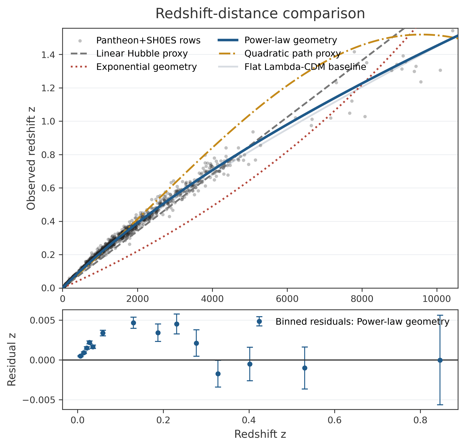
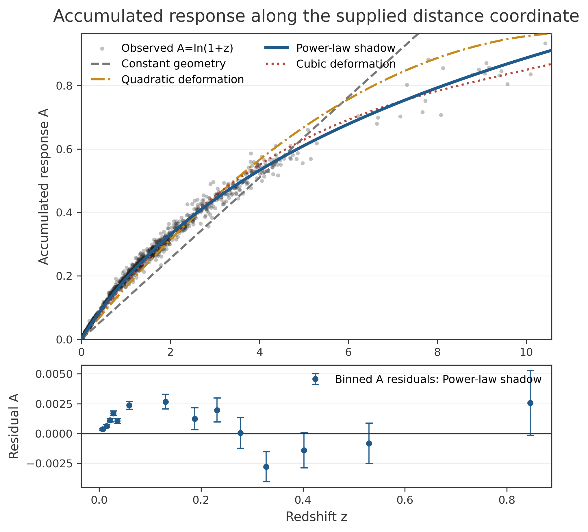
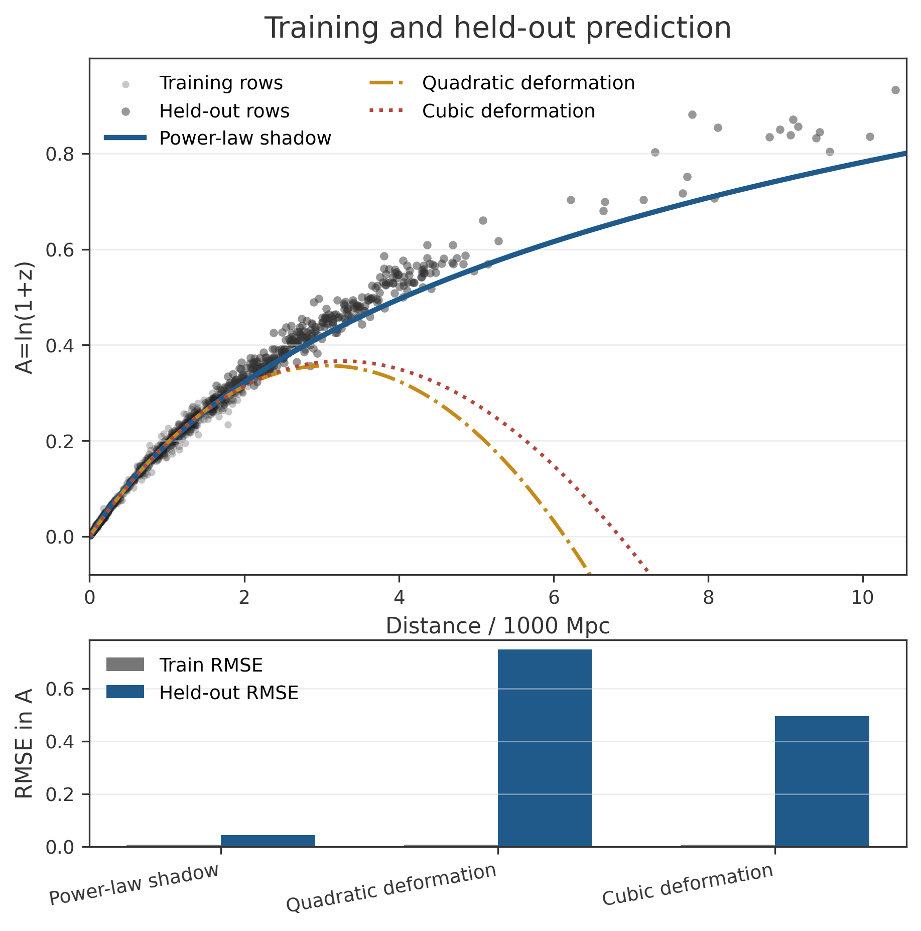
Using supplied supernova distance coordinates, the observed redshift was fit against linear, exponential, power-law, quadratic, and flat \(\Lambda\text{CDM}\) reference forms. These were ranked using residual patterns and standard statistical tools including RMSE, AIC, and BIC (Figure 1-2; [24]; [25]; [26]; [18]; [19]; [27]; [28]). Redshift is then rewritten as Equation (1-1) to track how the signal accumulates with path length (Figure 1-3). The power-law form was retained as it provides the most compact description of the observed curvature in this comparative analysis. All data were taken from published catalogues without re-fitting light curves or recalibrating distances [29] [30] [31].

**Figure 1-2.** Observed redshift vs. distance proxy \(d\), compared with various reference curves. The residual panel highlights the largest separation at high distances, supporting the selection of the power-law form as the starting relation.

\[A(d) = \ln(1 + z) \tag{1-1}\]

**Figure 1-3.** Redshift expressed as accumulated path response. By rewriting observed redshift as \(A(d)=\ln(1+z)\), the data is viewed as a quantity accumulated along the path. Residuals show where this transformation smooths the curvature and where structural anomalies remain.

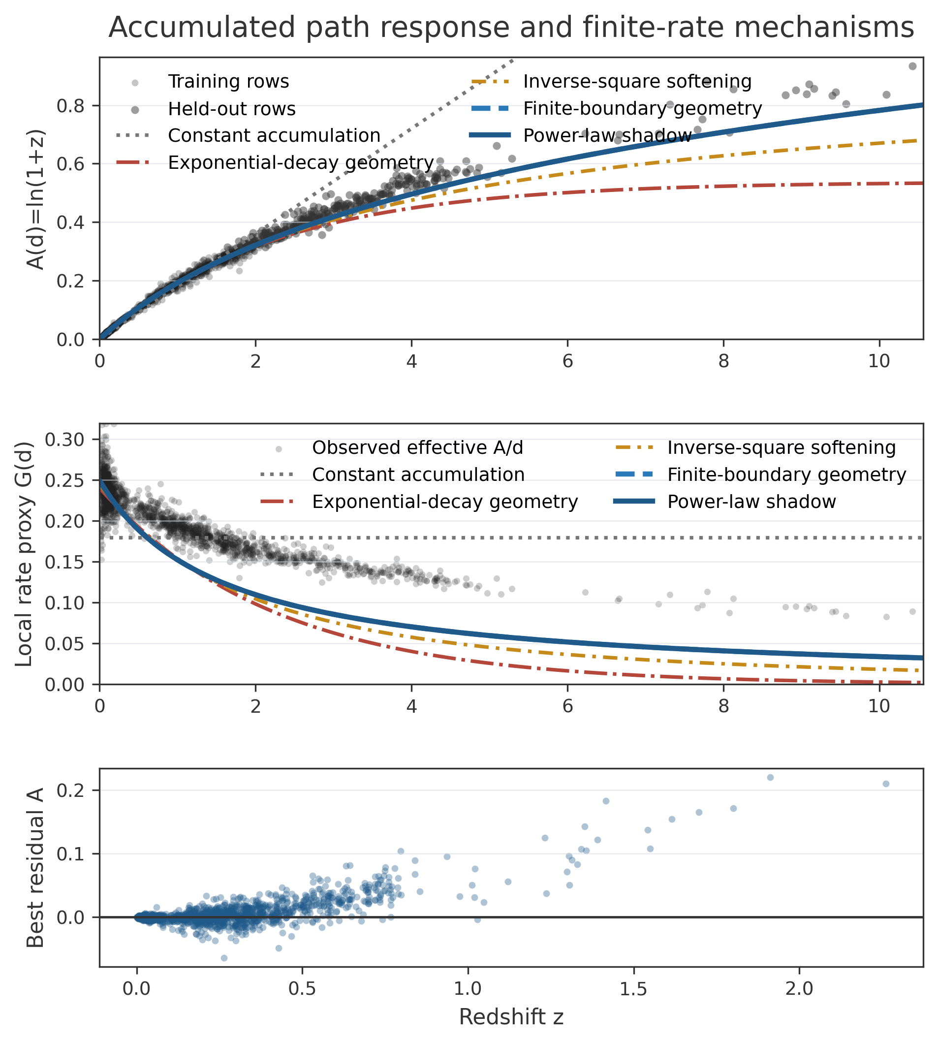
The finite-response law is expressed as the local-response law shown in Figure 1-4 and Equation (1-2):

\[G(d) = g_0 / (1 + d/d_b) \tag{1-2}\]

In this equation, \(d\) and \(d_b\) share distance units, \(g_0\) has inverse-distance units, and \(g_0 d_b\) is dimensionless.

See the Quantitative Appendix for units and derivation details.

Integrating Equation (1-2) yields Equation (1-3):

\[A(d) = g_0 d_b \ln(1 + d/d_b) \tag{1-3}\]

This result is converted back to redshift for observational comparison. The \(1/(1 + d/d_b)\) form is used as a phenomenological ansatz—the simplest monotonic weakening response that introduces one finite scale while maintaining logarithmic accumulation. The fitted scale \(d_b\) resides where Hubble-diagram curvature becomes visually significant; stability tests then determine if this scale persists across different datasets.

Stability and external comparison tests

To assess model generalization, five distinct probes are used: supernova luminosity distances, BAO ratios, cosmic chronometers, time-dilation measurements, and CMB distance priors [20] [21] [32] [33] [41] [22] [17]. Each probes a different physical question: supernovae provide the initial redshift-distance trend, BAO ratios probe standard ruler structure, chronometers probe derivative behavior, time-dilation probes temporal stretching, and CMB priors probe the high-redshift acoustic scale.

The analysis begins by checking the supernova trend against compact finite-response forms. The resulting scale \(d_b\) is then tested via resampling, catalogue changes, and sky partitions. Finally, the relation is compared against the other observables. If a shared BAO-CMB ruler fails, the analysis records the necessary recovery values \(S_{CMB}/S_{BAO}\) and \(T(z)\) required to resolve the mismatch.

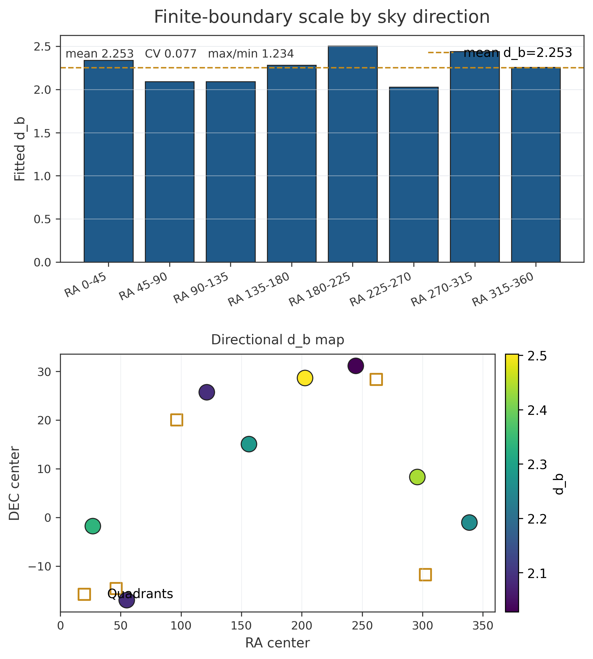
Cross-validation tests predictions for held-out points to ensure the model generalizes beyond the training subset (Figure 1-5; [34]). Redshift-window tests repeat the fit across various cutoffs and training fractions to determine the "win rate" and spread of the recovered \(d_b\) values (Figure 1-6). Dataset comparison checks if \(d_b\) is reproducible across independent catalogues, while sky-sector tests split the sample by quadrants and right ascension to check for directional isotropy (Figure 1-7).

For the external comparison set, the BAO analysis uses standard transverse, radial, and volume-averaged distance ratios tied to the sound-horizon scale through a nuisance parameter \(S\). The finite deformable relation is inserted into this ratio structure and compared with published values [35]. Because full covariance matrices were unavailable, \(\chi^2\) values are treated as shape-compatibility measures. The relation is also differentiated for chronometer comparisons and compared with published supernova time-dilation exponents (\(b\)), where \(b = 1\) represents full time stretching. Finally, Planck 2018 distance priors are combined with BAO distances via a shared-ruler calibration.

Scale-free BAO shape and recovery transition

The BAO anisotropy diagnostic provides a scale-free test of compatible scaling behavior [36] [37] [38] (Figure 1-11S). After normalization, the observable follows an approximately linear trend, summarized in Equation (1-8):

\[Q_{norm}(z) = 1.005z + 0.843 \tag{1-8}\]

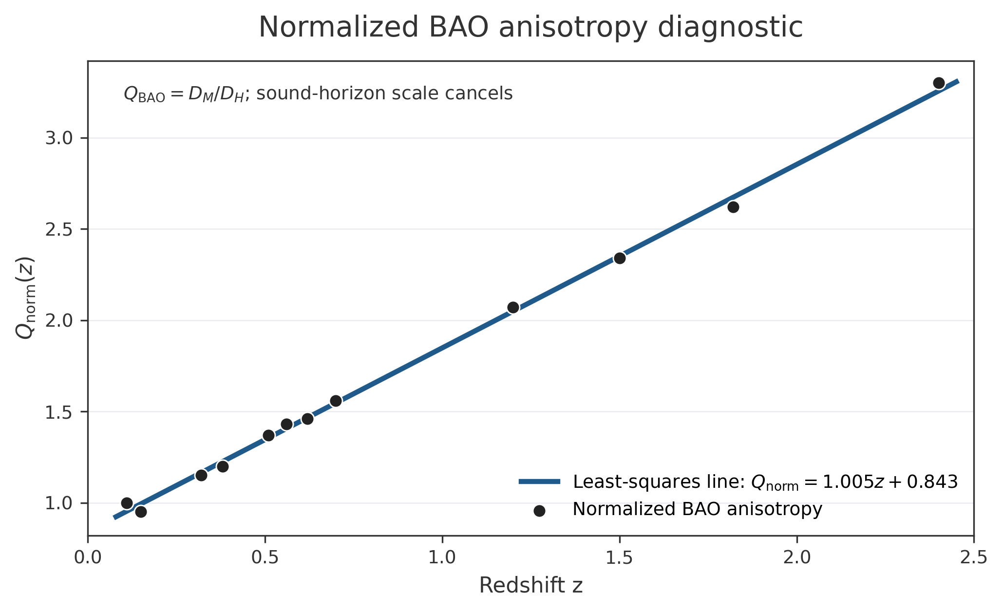
The near-unity slope indicates that the normalized radial-to-angular BAO observable grows linearly with redshift over the sampled range. This consistency suggests the BAO anisotropy shape aligns with the supernova power-law scaling without requiring further tuning. However, this remains a shape diagnostic; its statistical strength depends on the propagated uncertainties of the BAO data.

To diagnose the model's failure at the CMB scale, the projection function \(T(z)\) is used. Equation (1-7) provides the compact transition form used for the recovery target:

\[T(z) = 1 - \Delta z^m / (z^m + z_t^m) \tag{1-7}\]

In this function, \(T(z) = 1\) represents no projection change, \(1 - \Delta\) is the high-redshift asymptote, \(z_t\) is the transition midpoint, and \(m\) controls sharpness. This serves as a recovery target: the BAO range should remain nearly unchanged while the CMB-side projection shifts to the required compressed scale.

Results

Supernova curvature fits

The response law effectively organizes the supernova redshift-distance data [18] [19] [27] [28]. The power-law curve follows the observed curvature more closely than other empirical \(z(d)\) alternatives. Recasting this behavior into \(A(d)\) and \(G(d)\) reproduces the logarithmic buildup, although residual structure remains at higher redshifts.

Table 1-1 summarizes the main fit and constraint metrics, contrasting the local supernova results with the high-redshift shared-ruler failure.

Table 1-1. Summary metrics for the finite-response comparison.

Diagnostic	Flat \(\Lambda\text{CDM}\) / reference	Finite-response mapping	Comparator / note
Supernova RMSE	Not listed	Power-law: 0.0213	Linear Hubble: 0.0488; exponential: 0.1303; quadratic proxy: 0.0709
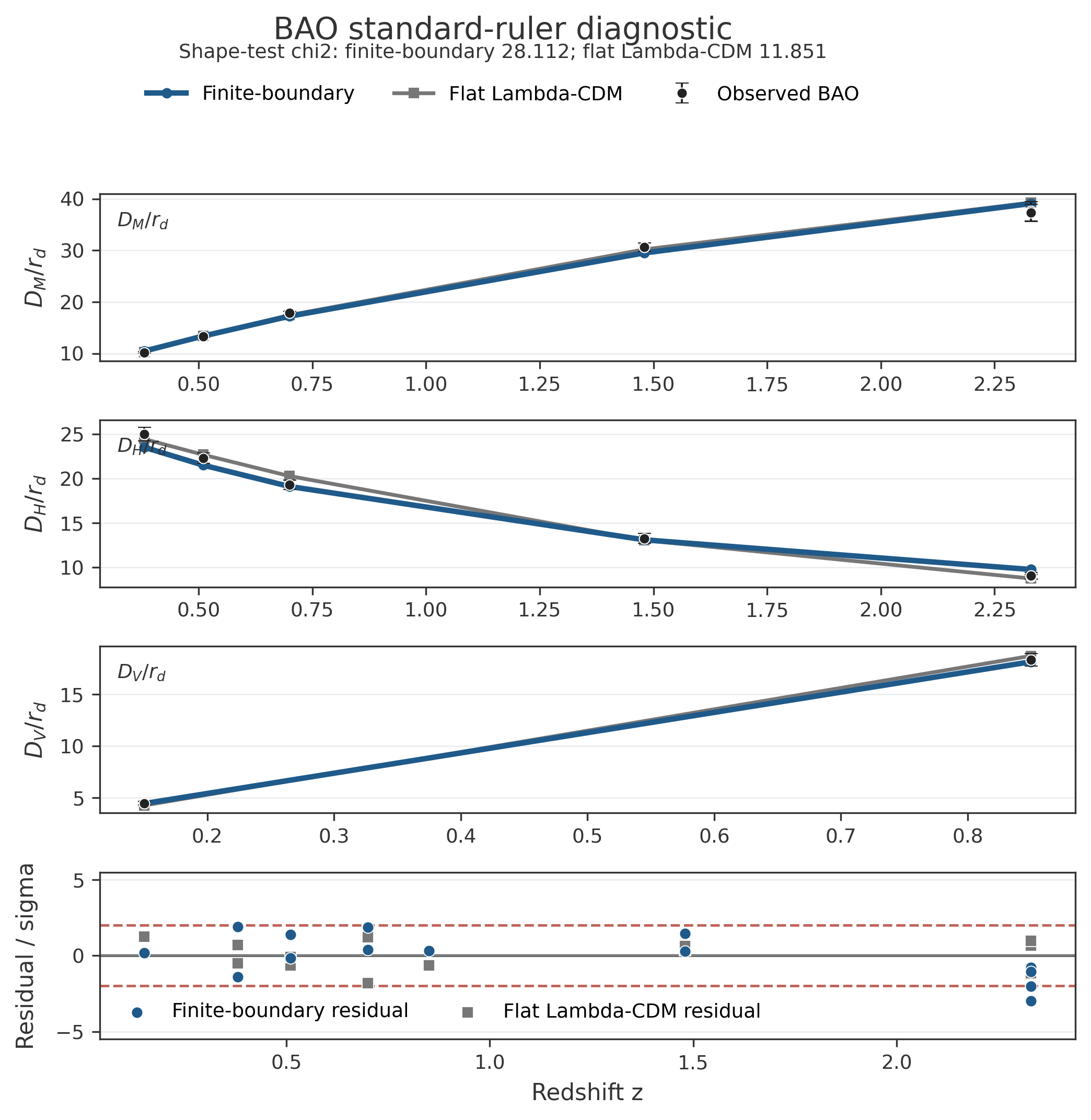
BAO shape \(\chi^2\)	11.8514	28.1117	Shape-comparison value; full covariance matrices not included
Shared-ruler total \(\chi^2\)	11.8573; red. \(\chi^2 = 0.9121\)	7732.7958	Finite-response mismatch is BAO dominated
Locked finite-ruler partition	N/A	BAO \(\chi^2 = 7730.6214\); CMB \(\chi^2 = 2.1744\)	Identifies the BAO-CMB shared-ruler failure

Data stability

Stability results indicate that low-redshift behavior is consistent across different data selections [27] [28] [39] [40]. In held-out predictions, the power-law relation outperforms constant-accumulation and polynomial alternatives. Redshift-window tests show a 97.6% win rate, with a median \(d_b\) near 1.57 and a coefficient of variation near 0.26. The Pantheon+SH0ES sample yields a \(d_b\) of approximately 2.32, while directional partitioning shows a mean \(d_b\) of 2.25 across right-ascension slices.

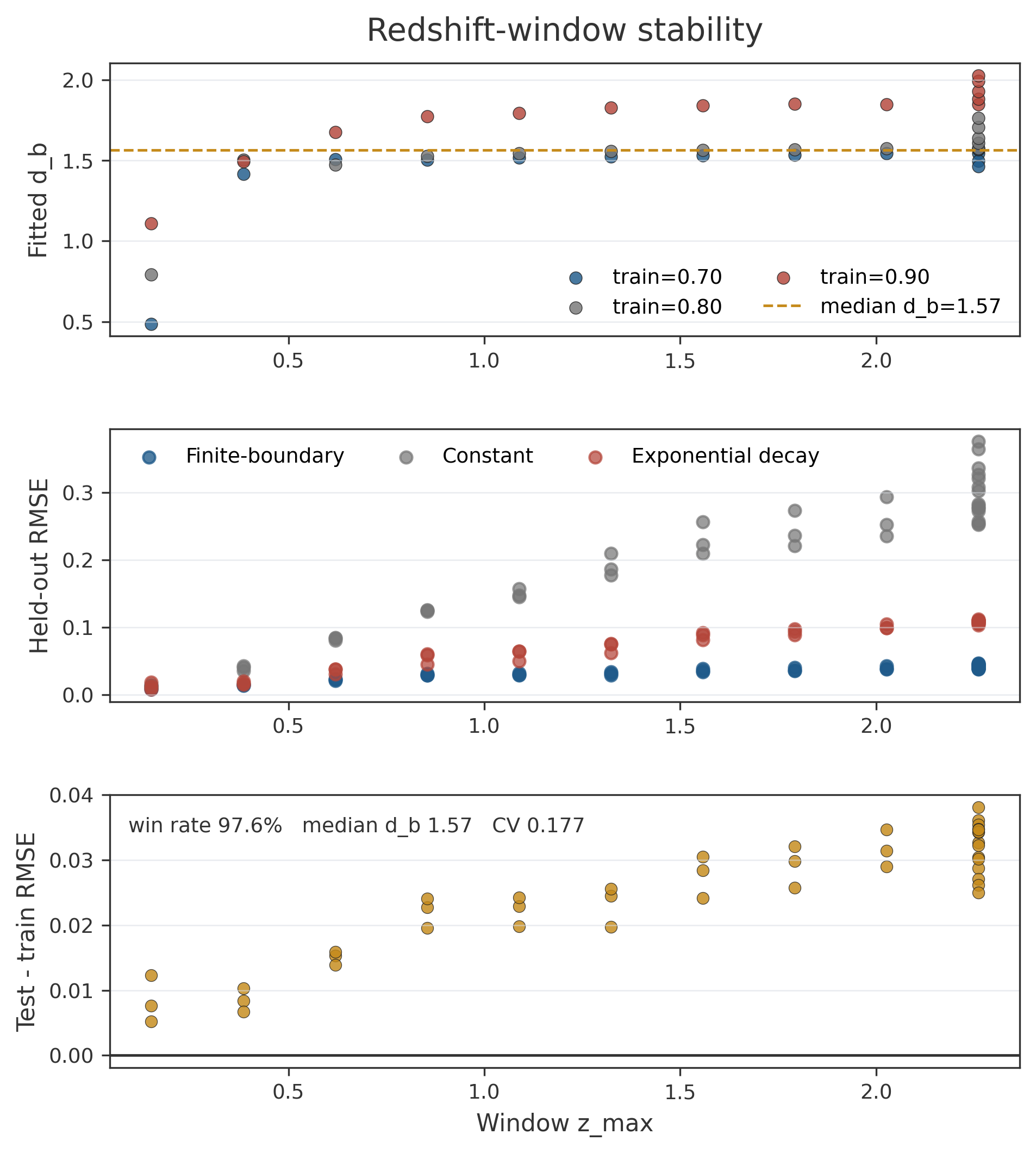
**Figure 1-6.** Robustness check of the fitted scale \(d_b\). The fit is repeated across various redshift cutoffs and training fractions, showing a 97.6% win rate and a median \(d_b\) near 1.57.

The shift in median \(d_b\) between resampling tests (\(\sim 1.57\)) and the Pantheon+SH0ES comparison (\(\sim 2.32\)) reflects sensitivity to catalogue definitions and redshift coverage. While this does not define a universal constant, the combined result is that the fitted scale remains finite and repeatable enough to support external checks.

**Figure 1-7.** Sky-sector fits comparing \(d_b\) across quadrants and RA-slices. A mean \(d_b\) of 2.25 and a low coefficient of variation (0.077) argue against a large directional breakdown.

BAO, chronometer, and time-dilation constraints

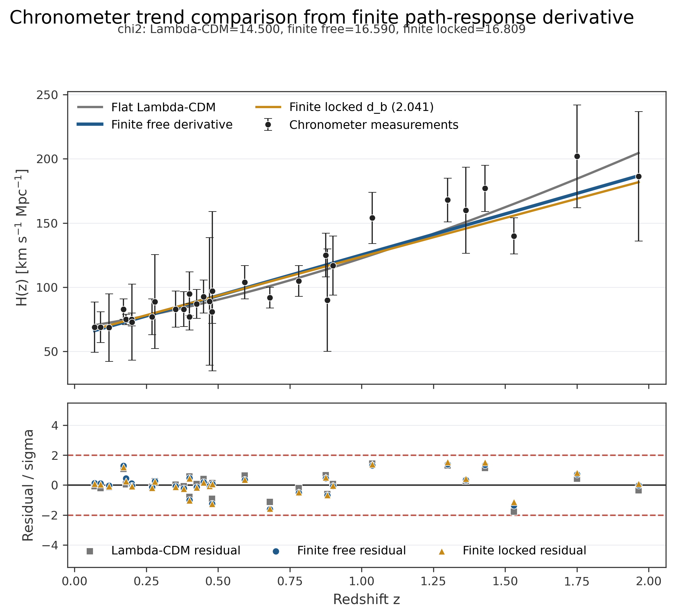
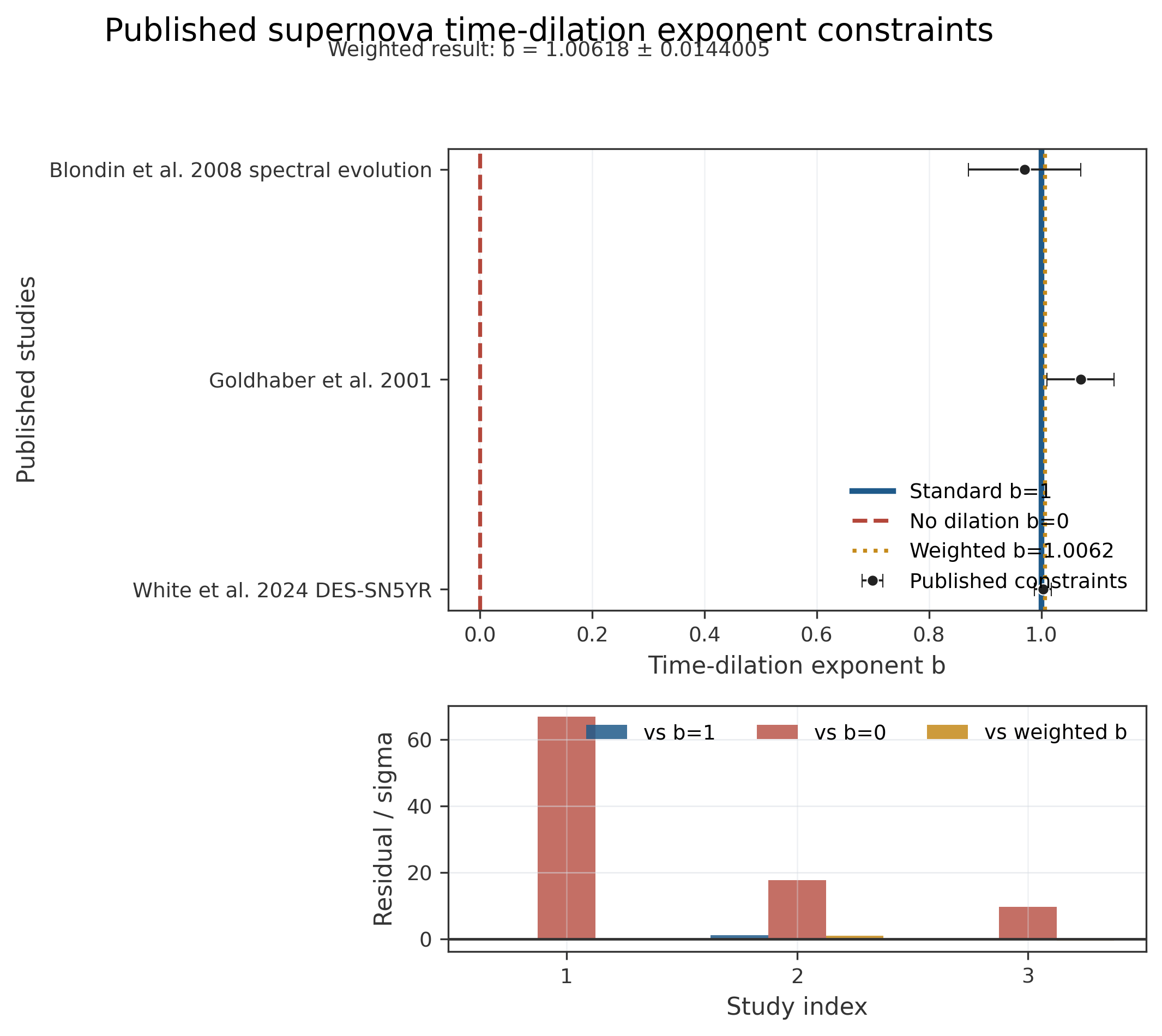
External data provides insights not visible in supernova comparisons [20] [21] [32] [33] [22] [17]. For BAO ratios, the simplified shape test yields \(\chi^2 = 11.8514\) for flat \(\Lambda\text{CDM}\) and \(\chi^2 = 28.1117\) for the finite deformable case (Figure 1-8), with the largest discrepancies found in radial BAO distances. Chronometer data follow the broad trend but remain sensitive to the locked \(d_b\) value (Figure 1-9). The weighted supernova time-dilation result remains close to \(b = 1\), confirming that any path-based redshift explanation must account for the stretching of photon-arrival intervals (Figure 1-10).

**Figure 1-8.** Conversion of the finite deformable distance coordinate into BAO ratios. Low-redshift points track well, while radial BAO and sigma residuals exhibit the highest tension compared to flat \(\Lambda\text{CDM}\).

**Figure 1-9.** The distance-redshift relation differentiated into an \(H(z)\)-style curve. Finite deformable variants follow the broad trend of differential-age chronometer measurements but vary based on the locked \(d_b\) value.

**Figure 1-10.** Comparison of published time-dilation exponents \(b\). The result near \(b = 1\) implies that any finite-geometry path-response must also include temporal stretching.

Scale-free BAO anisotropy

The Alcock-Paczynski-style BAO anisotropy check provides a scale-free test of compatible scaling behavior (Figure 1-11). After normalization, the observable follows an approximately linear trend, summarized in Equation (1-8):

\[Q_{norm}(z) = 1.005z + 0.843 \tag{1-8}\]

BAO-CMB shared-ruler failure and recovery target

The model's most significant break occurs when BAO and CMB information are forced to share a ruler scale [20] [21] [22] [23]. In this scenario, flat \(\Lambda\text{CDM}\) yields a total \(\chi^2 = 11.8573\), while the finite model with locked \(d_b\) yields a total \(\chi^2 = 7732.7958\), with the BAO portion dominating the mismatch. To resolve this, an effective scale ratio of \(0.390906\) is required between the CMB and BAO scales.

Equation (1-7) defines the recovery target needed to address this failure. The optimal recovery case employs \(\Delta = 0.627714\), \(z_t = 34.5754\), and \(m = 4\). This transition preserves the BAO range (\(T(2.3) = 0.999988\)) while dropping sharply to \(T(1089.92) = 0.372287\) at the CMB-side redshift. This identifies a sharp projection transition as the best recovery shape (Figure 1-12).

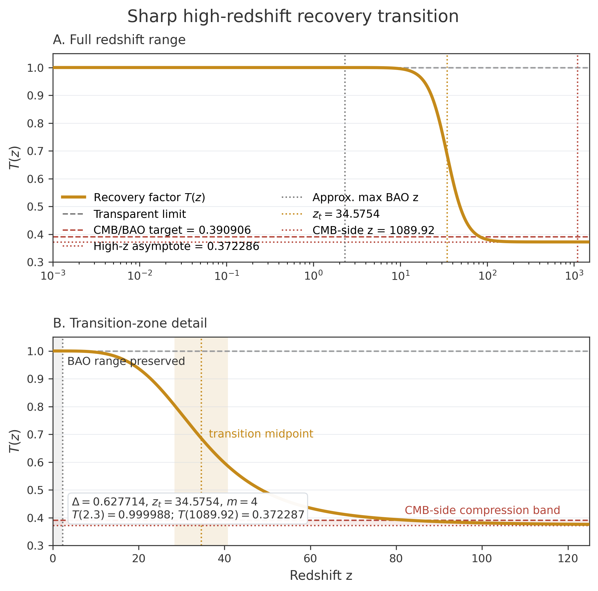
**Figure 1-12.** Reconstructed recovery transition for \(T(z)\). The function preserves the BAO redshift range and then drops sharply across an intermediate transition to match the CMB-side projection.

Table 1-2. Reconstructed boundary-layer recovery target.

Quantity	Value	Interpretation
\(\Delta\)	0.627714	Transition amplitude
\(z_t\)	34.5754	Transition midpoint
\(m\)	4	Transition sharpness (fourth-power form
\(1 - \Delta\)	0.372286	High-redshift asymptote of \(T(z)\)
\(S_{CMB}/S_{BAO}\)	0.390906	Separate-scale CMB-to-BAO effective ratio
\(T(2.3)\)	0.999988	BAO range remains essentially unchanged
\(T(1089.92)\)	0.372287	CMB-side projection approaches compressed band

High-redshift galaxy projection audit

The projection framework is further evaluated using JWST high-redshift galaxy data. Labbé et al. (2023) [42] reported red candidate massive galaxies at \(z \approx 7.4\)–\(9.1\), and Baggen et al. (2023) [43] measured their effective radii. This audit uses eight objects with both published stellar-mass estimates and effective radii [44] to determine if a finite-geometry projection shift moves these properties in a theoretically expected direction.

To evaluate the model's sensitivity, a fourth-power shoulder centered in the JWST redshift range was used. The amplitude \(\Delta = 0.627714\) was retained from Equation (1-7), but the midpoint was shifted to \(z_s = 8\) to determine if a weaker shoulder affects the red massive galaxy regime:

\[\Phi(z) = 1 - \Delta z^4 / (z^4 + z_s^4) \tag{1-9}\]

The audit then recalculates derived quantities: flux-based mass (which scales with luminosity-distance squared) and physical radius (which scales through the angular-size-distance register). The projection factor is used as a diagnostic scaling (detailed in the quantitative appendix):

See the Quantitative Appendix for diagnostic mass-size scaling details.

\[M_\star(audit) \approx \Phi(z)^2 M_\star(\Lambda\mathrm{CDM}) \tag{1-10}\]

\[Re(audit) \approx Re(\Lambda\mathrm{CDM}) / \Phi(z) \tag{1-11}\]

The results are consistent across the sample (Table 1-3; Figure 1-13). The median log stellar mass shifts from 9.7369 to 9.4260, the median effective radius increases from 125.5 pc to 190.0 pc, and the median compactness proxy falls from 5.4826 to 4.9411. The significant point is the direction of the response: the projection correction required by the acoustic-scale failure also moves high-redshift galaxy properties in the direction needed to reduce the "too massive and too compact" tension.

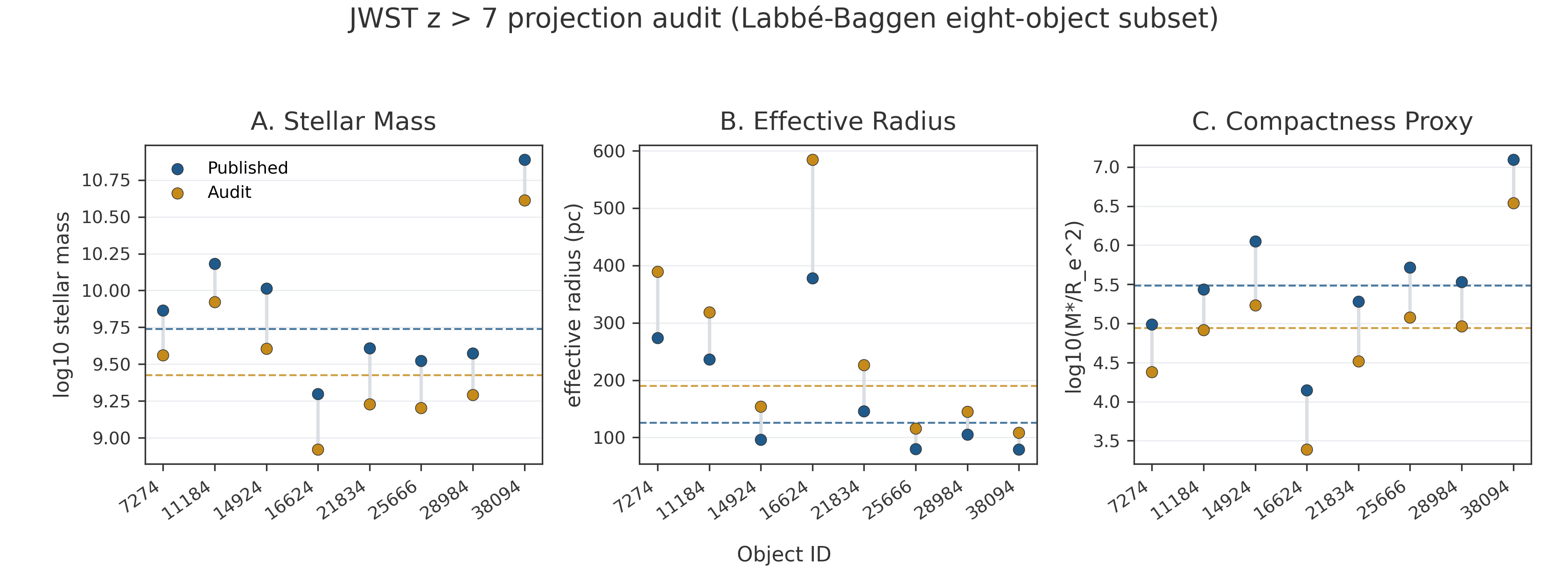
Table 1-3. JWST \(z > 7\) projection-audit summary.

Quantity	Published \(\Lambda\text{CDM}\) median	Finite-geometry audit median	Direction of change
Median log stellar mass	9.7369	9.4260	Lower mass
Median effective radius (pc)	125.5	190.0	Larger size
Median log compactness	5.4826	4.9411	Lower compactness

The sample is small because it requires both mass estimates and structural radii from the same candidates. Future tests should employ spectroscopic redshifts and homogeneous SED modeling.

Discussion

What the finite deformable mapping captures

Supernova tests provide the strongest support for the proposed response law. In this regime, the law captures observed curvature with a compact, declining-response form and remains stable across holdout and directional tests. This establishes a specific fitted relation that can be tested against independent distance and time-domain observables.

The Alcock-Paczynski-style BAO anisotropy result adds independent shape context. A comparable scaling appears when BAO information is reduced to a radial-to-transverse shape ratio. However, this does not resolve the shared-ruler failure: the model may capture the scale-free BAO shape while still failing the absolute calibration that connects BAO measurements to the CMB acoustic scale.

What breaks

The primary difficulty arises from the BAO and CMB data. A ruler calibration that works across the BAO range does not automatically satisfy high-redshift acoustic-scale priors. The limiting issue is not the supernova fit, but the single-ruler link between the BAO and CMB regimes.

Boundary-layer projection interpretation

The boundary-layer projection offers a contrast to the common theoretical resolution for the BAO-CMB failure: Early Dark Energy (EDE) [45] [46]. EDE models modify the early universe by introducing a scalar-field energy component near matter-radiation equality (\(z \approx 3000\)) to reduce the physical sound horizon. In contrast, the finite deformable framework does not modify early plasma physics or expansion history. Instead, it attributes the calibration failure to a geometric projection effect occurring much later, near \(z \approx 35\)–\(37\). The absolute size of the acoustic ruler is not changed; rather, the mapping between redshift and inferred distance shifts across a regime boundary.

Projection tests indicate that a broad rescaling would move the curve in the wrong direction. A successful mechanism must leave the BAO sector nearly unchanged while producing a rapid change in projection across an intermediate-redshift transition. \(T(z)\) represents this required "bend" in the model. This mechanism must also account for the observed stretching of photon-arrival intervals; a simple relabeling of distance or wavelength would not suffice.

The reconstructed transition points to a boundary-layer projection. Wavelength and arrival-time stretching remain tied to the accumulated path response, but the mapping between redshift and standard ruler distance changes. In this interpretation, time, distance, and wavelength are observational registers of a shared deformable geometry. Their relationships are stable within a regime but shift when signals cross a projection boundary, making inferred distances and velocities between widely separated galaxies regime-dependent.

The recovery curve now sets a concrete target for theory: a physical model must explain why the transition midpoint is near \(z_t = 34.5754\), why it has a fourth-power shape, and why it preserves BAO-scale projections while landing near the CMB-side compression band.

Technical note

The high-redshift asymptote of the recovery function, \(1 - \Delta = 0.372286\), is close to \(e^{-1} = 0.367879\). If \(T(z)\) is later interpreted as an attenuation or transmission factor, this would correspond to roughly one characteristic attenuation length.

High-redshift galaxy implication

The JWST audit provides a separate direction-of-effect check. By recalculating observed redshift, flux, and angular size using the finite-geometry projection, the inferred galaxies appear less massive, larger, and less compact. This tests whether luminosity distance and redshift remain locked to expansion-based conversions at early cosmic times.

Limitations

Methodological limits remain. Full BAO and CMB inferences are covariance-sensitive, and compressed CMB priors do not carry the full anisotropy spectrum. The BAO comparison omits covariance matrices, and the response law currently lacks a first-principles dynamical derivation. While the Alcock-Paczynski ratio cancels the absolute sound-horizon scale, published measurements still depend on survey modeling and fiducial cosmology conversions.

Overall, the analysis identifies a phenomenological response relation, a scale-free BAO shape check, a shared-ruler failure, and a sharply defined recovery target. Any physical finite-geometry mechanism must meet these numerical requirements.

Conclusion

The accumulated-response form successfully organizes the Type Ia supernova redshift-distance relation and remains stable under internal tests. The Alcock-Paczynski-style BAO anisotropy diagnostic yields \(Q_{norm}(z) \approx 1.005z + 0.843\) once the absolute ruler scale is removed. However, under a shared BAO-CMB ruler calibration, the mapping breaks sharply.

The recovery target requires a narrow transition (\(\Delta = 0.627714, z_t = 34.5754, m = 4\)) that preserves the BAO range while producing a high-redshift projection change close to the magnitude isolated by separate-ruler tests. Future physical models must explain this specific transition behavior.

Finally, the JWST \(z > 7\) audit demonstrates that when published masses and radii are recalculated with a finite-geometry projection shoulder, inferred masses and compactness decrease while effective radii increase. This result motivates further high-redshift galaxy tests using homogeneous spectroscopy and morphology.

Reader note: The redshift-path idea fits the supernova pattern in a useful way, but it does not carry every test by itself. The chapter ends with a concrete demand: any stronger model must explain a sharp change in how distant observations are translated, while preserving the successful lower-redshift behavior.